PathTracer

Part 1: Ray Generation and Intersection

For task 1, I first implement the special case when ns_aa == 1. In this case, a ray is generated through the center of the pixel. To get the center of the pixel, 0.5 is added to both the x-and y-coordinates of the "origin" of the pixel (which is the bottom left corner of the pixel), and then divided by the width and height (respectively) of the SampleBuffer to scale the x-and y-coordinates to [0,1]^2 coordinates. Then camera->generate_ray(...) is called on those coordinates to get the ray. And finally, trace_ray(...) is called to trace that ray.

In the normal case where ns_aa > 1, I first declare a running Spectrum variable. Then, iterating ns_aa number of times, a sample coordinate is generated by gridSampler->get_sample(). Like before, the sample coordinates are added to the x-and y-coordinates of the origin of the pixel (respectively) and divided by the width and height (respectively) of the SampleBuffer. camera->generate_Ray(...) is called with the [0,1]^2 coordinates to create a ray, and trace_ray(...) traces that ray. The return value trace_ray(...) (a Spectrum) is added to the running Spectrum variable at each iteration. At the end, the running variable is divided by ns_aa to return the averaged Spectrum value for the given pixel.

In task 2, I implement generate_ray(...). First, I find the bottom left and top right corners of the viewing plane in camera space. Then, the difference between these two corners is taken, which gives a vector whose x-component describes the width of the viewing plane and y-component describes the height of the viewing plane. Using the passed in [0,1]^2 coordinates, I scale the width-difference and the height-difference, and add those scaled differences to the bottom left corner's coordinates. This gives the ray's direction in camera space, or also the location on the viewing plane which the ray intersects. This location-vector in camera space is then converted to world coordinates, which gives the ray's r.d direction value. The ray's r.o is the position of the camera. r.min_t and r.max_t are assigned nClip and fClip respectively, which are the minimum and maximum bounds for possible intersection-time values.

In task 3, I use the Moller Trumbore algorithm to test for ray intersections with triangles. I first compute the 4 scalar triple products required for computing the intersection time, t, barycentric coordinate 1 of the triangle, b1, and barycentric coordinate 2 of the triangle, b2. Scalar triple products are equivalent to finding the determinant of a 3x3 matrix composed of 3 horizontal 3-vectors. The first scalar triple product serves as a scaling/normalizing factor to the other products: it is the determinant of (ray's direction), (triangle edge 1), (triangle edge 2). The intersection time, t is given by dividing the [determinant of (vector of triangle vertex 1 to ray's origin), (triangle edge 1), and (triangle edge 2)] by the previous scaling factor. Then, b1 is found by dividing the [determinant of (ray's direction), (triangle edge 2), and (vector of triangle vertex 1 to ray's origin)] by the previous scaling factor. Finally, b2 is found by dividing the [determinant of (vector of triangle vertex 1 to ray's origin), (triangle edge 1), and (ray's direction)] by the previous scaling factor.

If time t is out of bounds, then false is returned. If any of the barycentric coordinates b1, b2, or 1-b1-b2 are less than 0 (out of bounds), then false is returned. Otherwise, r.max_t is set to the intersection time and true is returned. r.max_t is set so that objects in the fore or back of another object are correctly covering or being covered by the other object. That is, things in front of other things actually show up like that. If an Intersection pointer was passed in, the Intersection variable is updated to contain the new information: time, primitive, normal, and bsdf. The normal is an interpolation of the vertex normals using the barycentric coordinates.

For task 4, in Sphere::test(...), I test to see if a ray intersects with the given Sphere object. The time-based formula of a ray is set to equal the formula of a sphere, and the variable of time, t, is solved for. t is given by evaluating the quadratic formula with a = dot(r.d, r.d); b = 2 * dot(diff, r.d); and c = dot(diff, diff) - this->r2. The discriminant of the quadratic formula is evaluated first (b^2 - 4ac). If the discriminant is negative, there is no intersection and false is returned. Otherwise, one or two solutions exists (if discriminant == 0 or discriminant > 0 respectively). The solutions to the quadratic formula are evaluated fully. The two time solutions are swapped such that t1 is always smaller than t2. Given that there are time solutions to the intersection, in Sphere::intersect(...) we then check to make sure both intersection times are within bounds. If not, false is returned. If it is within bounds, true is returned. If an Intersection pointer was passed in, its values are updated: time, primitive, normal, and bsdf. The normal is the unit vector pointing from the sphere's center to the first intersection point. At first, I had some errors in calculating the normal vector's direction correctly.

Part 2: Bounding Volume Hierarchy

Implementing a Bounding Volume Hierarchy (BVH) reduces the rendering from linear time to log time. This allows scenes with hundreds of thousands of primitives to be rendered in a reasonable amount of time. Rendering CBlucy.dae, which has 133796 primitives, only took 20.5226 seconds. And, rendering dragon.dae, which has 105120 primitives, took 19.5581 seconds.

To render a scene, a BVH is first constructed from the scene's primitives. The BVH I implemented is a binary tree: each non-leaf node (interior node and root) points to a left and a right child node; each leaf node contains a vector of primitives. All nodes have a BBox, an object which contains information about the bounding box of all primitives under that node. The BVH is recursively constructed. For the base case, if the number of primitives passed in is less than a given max_leaf_size, that node is a leaf. It has a vector of the primitives that were passed in, a bounding box, and no child nodes. The leaf node is returned.

Otherwise, the node is not a leaf (and is interior), and the vector of primitives that are passed in are split into two separate vectors of primitives; the bounding box of the node is created; and the left and right child nodes are created. The two separate vectors of primitives are recursively passed into contruct_bvh and the returned nodes are assigned to be this node's two child nodes. The two separate vectors of primitives are intended to be approximately equal in size. The initial vector that was passed in, is sorted into the two separate vectors by: first getting the axis of the longest side of the bounding box, second finding the "reference" centroid of the bounding box of the primitives' respective centroids, and then sorting the primitives by their centroids in relation to the reference centroid. (Split point = centroid_box.centroid().longest_axis). For the rare case where the sorting creates one new vector that is equal in length to the initial vector and the other new vector is empty, this interior node becomes a leaf node. All of the primitives are simply collected into this node's vector and no child nodes are created. This final resulting node, leaf or not, is returned.

For intersecting a BVH, I first implement intersection of a bounding box, BBox::intersect(...). First, I find the intersection times of the ray with the two x-axis-oriented planes of the bounding box.

( For any axis w (x/y/ or z), if r.inv_d.w >= 0, then [time of first intersection tw1 = (min.w - r.o.w) * r.inv_d.w] and [time of second intersection tw2 = (max.w - r.o.w) * r.inv_d.w]. Otherwise if r.inv_d.w <= 0, then [time of first intersection tw1 = (max.w - r.o.w) * r.inv_d.w] and [time of second intersection tw2 = (min.w - r.o.w) * r.inv_d.w]] )

And then I also find the intersection times of the ray with the two y-axis-oriented planes of the bounding box. I know that if (tx1 > ty2) or (tx2 < ty1), there is no intersection with the bounding box, and return false. Otherwise we have (tmin = min(tx1, ty1)) and (tmax = max(tx2, ty2)). I then find the intersection times of the ray with the two z-axis-oriented planes of the bounding box. I know that if (tmin > tx2) or (tmax < tz1), there is no intersection with the bounding box, and return false. Otherwise we have (tmin = min(tmin, tz1)) and (tmax = max(tmax, tz2)). Finally, if false has not been returned already, the passed in references (to = tmin) and (t1 = tmax), and true is returned. The ray's min_t and max_t variables are not set here, as doing so will wrongly restricted the time boundaries: this makes it so that testing the intersection of the bounding box of a right child node incorrect after testing the intersection of the left child node.

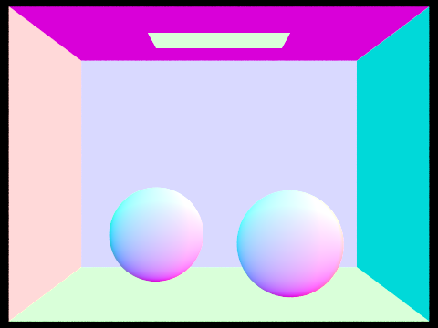
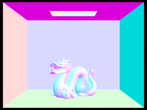
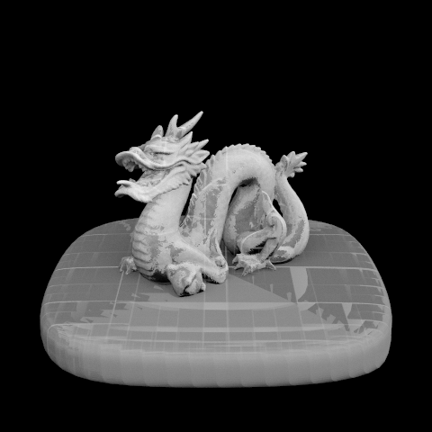
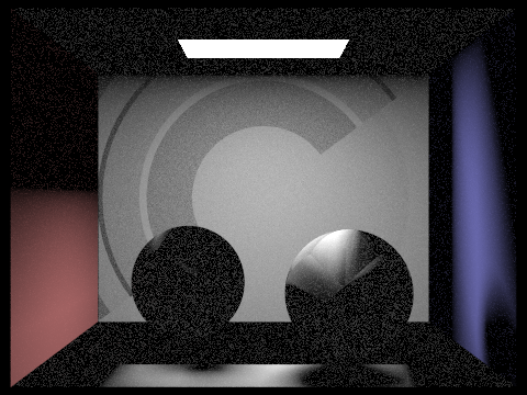
For the BVHAccel::intersect(...), this function is also recursive. First, the ray is checked to see if it intersects with the bounding box of this node, using BBox::intersect(...). If it does not, immediately return. Otherwise, check if the current node is a leaf node. If it is a leaf node, iterate through this node's vector of primitives, and find the intersection with the lowest intersection time. (That is, set the passed in *i to have the data of the Intersection tempI with smallest tempI.t of all the primitives.) After *i is updated with the data of the shortest Intersection time, true is returned. False is returned if none of the primitives are actually intersected. The ray's min_t and max_t values, and total_isects, are set appropriately. Otherwise if it is not a leaf node, then we recurse by calling BVHAccel::intersect(...) on the left AND the right child of this node. A bug arose here, which is shown in the first picture below: my furthest away intersections were being rendered in front of my closest intersections. This bug is because I passed in the same Intersection *i pointer into both recursive calls, causing the second recursive call to overwrite *i of the first recursive call. The fix was to have a temporary Intersection tempI. I pass the reference of tempI into BVHAccel::intersect(...), and then only set the data of Intersection *i to have the data of tempI if (tempI.t < i->t). That is, only update i after each recursive call if the new Intersection tempI has a shorter time than the current i. If Intersection *i is updated after either recursive call, true is returned; otherwise there was no intersection and false is returned.

Part 3: Direct Illumination

In implementing direct lighting, we first calculate the world coordinates of the hit point, which is where the given ray intersects with the surface primitive. Then a Spectrum varaible is created for L_out, which is the total outgoing radiance at this hit point. For this hit point, all of the SceneLights in the scene are iterated over. For each scene light, if it is a delta light, we only need to sample it once, since the values of the samples are all uniform. Otherwise, we sample ns_area_light number of times for the current scene light. Then for each light sample (1 or more than 1 samples per SceneLight), we call SceneLight::sample_L(...) using the hit point as a parameter. This function returns the incoming radiance, a world space vector from the hit point to the light source, the time-based distance from the hit point to the light source, and the probability density function evaluated at that vector's direction. Then, we check that the z-coordinate of the object space version of the vector from the hit point to the light source is positive; this is to make sure the light source is on the correct side of the surface. If it is, we continue through the loop, otherwise, we skip to the next iteration of SceneLight. Continuing through the loop, we then contruct a shadow ray from the hit point to the light source. This shadow ray originates at the hit point plus an offest of (Epsilon * world space vector from hit point to light source). The offset origin of the shadow ray is included to avoid numerical precision issues: precision issues might cause a shadow ray to start behind its own surface and intersect its own surface, leading to a false intersection. The shadow ray goes from the offset hit point towards the light source, with a maximum time of (distance to light). The purpose of this shadow ray is to check whether there is another object between this hit point and the light source: if there is, then the hit point is a shadow and it's radiance is not included into the running L_out. If the shadow ray does not intersect another object, the current hit point is illuminated by the light source, and we therefore include the Spectrum value returned by isect.bsdf->f(...) in the running L_out. The bsdf at this hit point is calculated using the using the object vectors w_out and w_in. Finally, we have:

$$L_{out} += (sample\_L * w\_in.z) * (bsdf\_val \div pdf) \div ns\_area\_light$$

We accumulate the radiances into L_out. Sample_L contains an incoming radiance, it is converted to an irradiance using a cosine term: (w_in.z). w_in.z is a cosine term because it is the dot product of the two unit vectors w_in and (0,0,1). The bsdf_val is multiplied to the scaled sample_L. And the whole expression is divided by pdf to undo bias resulting from the probability distribution of sampling the light. And that whole expression is divided again by ns_area_light, so that the final L_out (after accumulating and dividing) is correctly averaged over all of the light samples. In the case of a delta light, ns_area_light == 1, so there is no need to divide by the number of samples there.

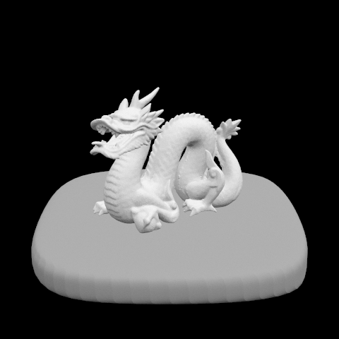
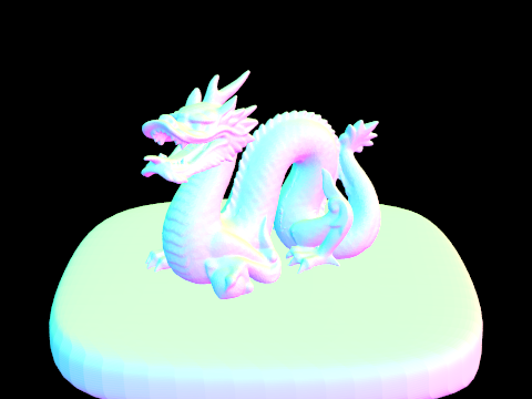
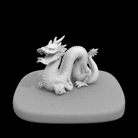
Comparing the 4 dragon images below. All of the images used 64 camera rays per pixel. The first dragon used 1 sample per area light, the second dragon used 8 samples, the third used 32 samples, and the fourth used 64 samples. The first image does have some graininess to it. The surface of the model looks like it has a rough, rocky texture. The lighted areas and shadow areas of the image are not well contrasted. Shadow borders are fuzzy. In the second image, the surface appears smoother than before, but there is still some graininess to the image. The edges of the shadow appear to be better defined, but there is still moderately low contrast between light and shadow. In the third image, the surface of the model looks smooth, now without tiny speckles. The contrast between lighted surfaces and shadows is much more prevalent than before, and borders are pretty well defined. The fourth images looks very similar to the third image. I can only perceive that this image has a very-very-slightly more contrast between lights and darks than the previous image.

Part 4: Indirect Illumination

In implementing indirect lighting, I first declare a (black) Spectrum s, which will hold the recursive result of calling trace_ray(...) later. Then, a Spectrum is assigned to hold the result of sampling the surface BSDF at the intersection point. That is, bsdf_val holds the Spectrum returned by isect.bsdf->sample_f(...). Sample_f also returns the probabilistically sampled w_in unit vector of the object's incoming radiance direction, and the probability density function pdf evaluated in that direction.

Then I calculate the Russian roulette probability of this ray terminating. To do this, I took the reflectance of the bsdf_val Spectrum (bsdf_val.illum()) and divided it by 255.0. This is because illum() returns a weighted sum of rgb values of the spectrum, outputting a float with value [0.0, 255.0]. Dividing illum by 255.0 reduces the range to [0.0, 1.0]. Then I multiply illum by a large constant of 10 to make sure that the rays are not terminating too early, which could result in high noise. The new range of [0.0, 10.0] is clipped to [0.0, 1.0] using std::max(0.0, std::min(illum, 1.0)). So all values (1.0, 10.0] are simply 1.0. The final value in the range [0.0, 1.0] is the calculated Russian roulette probability. A coin is then flipped using coin_flip(roulette) to see if this ray terminates on this function call or if the ray continues to recurse. Since coin_flip returns whether a uniform random is less than roulette's value, and roulette is often clipped at 1.0, there is a very low chance of termination per call - so that rays do not terminate too early.

If the ray is terminated, the black Spectrum s is simply returned. Otherwise, the ray continues on its recursive path. The w_in calculated from sample_f(...) is converted to wi, the world coordinate counterpart of the incoming radiance direction. A newRay is created, originating at (hit point + offset), directed towards, with a max time of r.max_t, and a depth of (r.depth - 1). The offset to the hit point here is (EPS_D * o2w * Vector3D(0.0, 0.0, w_in.z)). Unlike in direct illumination, we offset by the normal vector to the surface instead of w_in: w_in.z is the object coordinate of the surface normal, so o2w converts that vector to its world coordinate form. The newRay is recursively passed into trace_ray(newRay, isect.bsdf->is_delta()). (Recursively because trace_ray(...) down the line calls estimate_indirect_lighting(...).) (We pass in isect.bsdf->is_delta() since emission is not part of direct light calculations for delta BSDFs.) The result of trace_ray is recorded into Spectrum s. Finally, a scaled Spectrum s is returned.

return(s * bsdf_val * w_in.z) / (pdf * (1 - roulette))

The incoming radiance s in converted to the outgoing radiance estimator (to be returned) by scaling it with the BSDF and the cosine factor (as in Part 3). And then it is divided by the BSDF's probability density function (to remove bias), and divided again by (1 - Russian roulette termination probability). The (1 - roulette) is the chance that the ray did not get terminated.

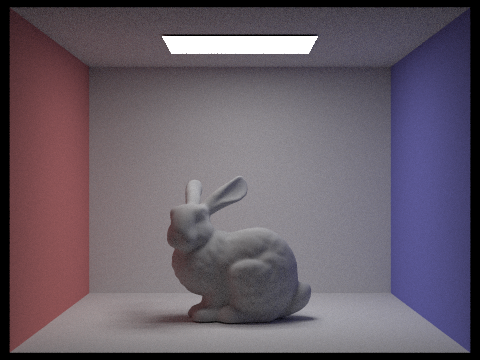
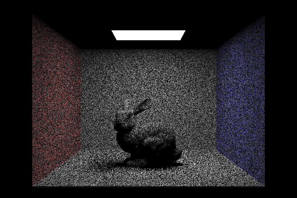
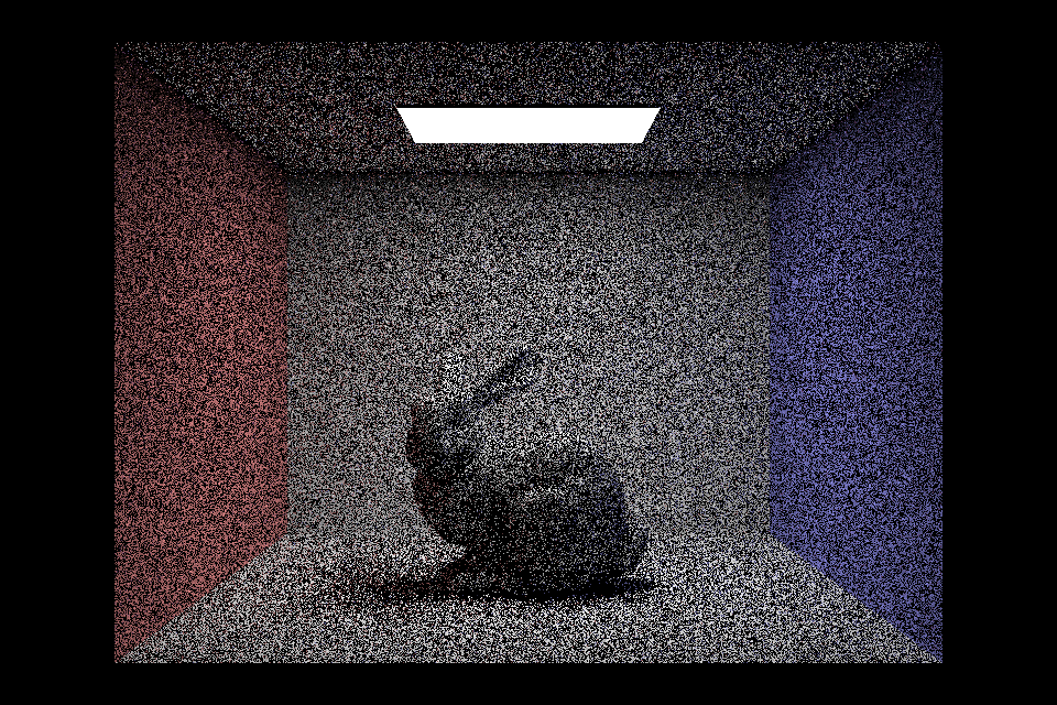
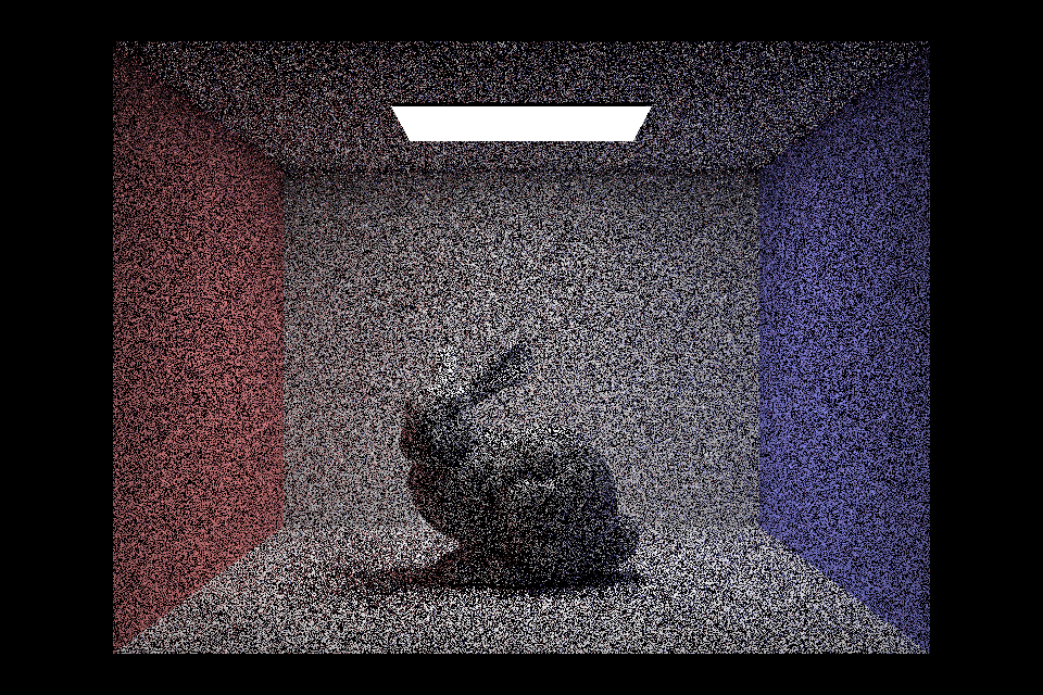
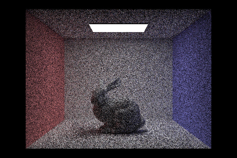
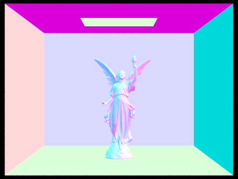
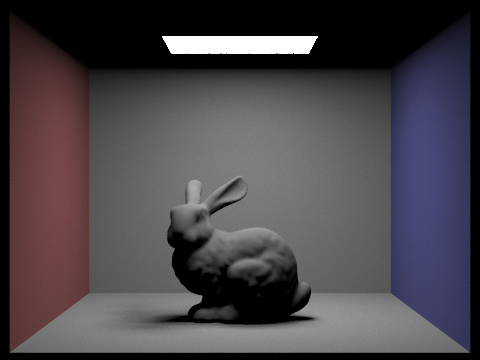
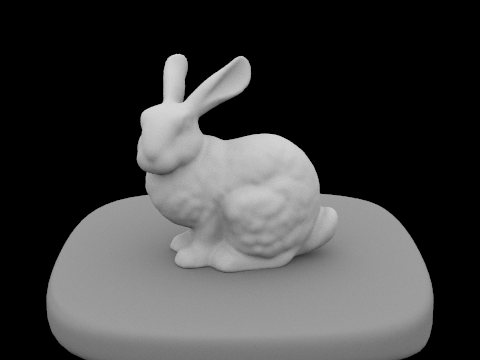
This is what I have implemented, and I have followed the spec as closely as I could tell. However, my end result (the bunny below) still had some visual glitches and bugs. I have hunted for this bug for many hours, but still could not resolve it.

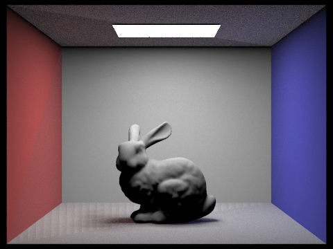
I did not have enough time to render each step to full quality, as each picture here takes over one hour to produce on an old Macbook Air. The lower ones would take multiple hours per full quality render.