There are many differences between a pinhole camera (as in the previous project) and a fully simulated lens system (as in this project). Firstly, a pinhole camera has no lens, and in real life, a pinhole camera is subject to light diffraction effects. A lens system can converge light without reducing the amount of light in the scene. Using a lens system, a camera can focus on individual objects and blur other parts of the scene. Unlike a pinhole camera, a lens camera has a variable aperture, which allows the amount of light coming into the sensor to be adjusted. Also unlike a pinhole camera, a lens camera has adjustable perspectives, for example, one can have wide angle lenses, fisheye lenses, or telephoto lenses, all of which have different effects on the image. The wide angle lenses capture more horizontal space in the world, fisheye lenses capture a wide hemisphere of the world, and telephoto lenses capture far away (small angle) images of the world. Additionally, lens cameras can produce aberrations, such as circles of confusion and bokeh. Lenses can also be manipulated during the capturing of an image to produce interesting effects, like tilt-shift photography, which makes scenes appear minature. In real life, both pinhole and (single) lens cameras capture images upside-down to the world.
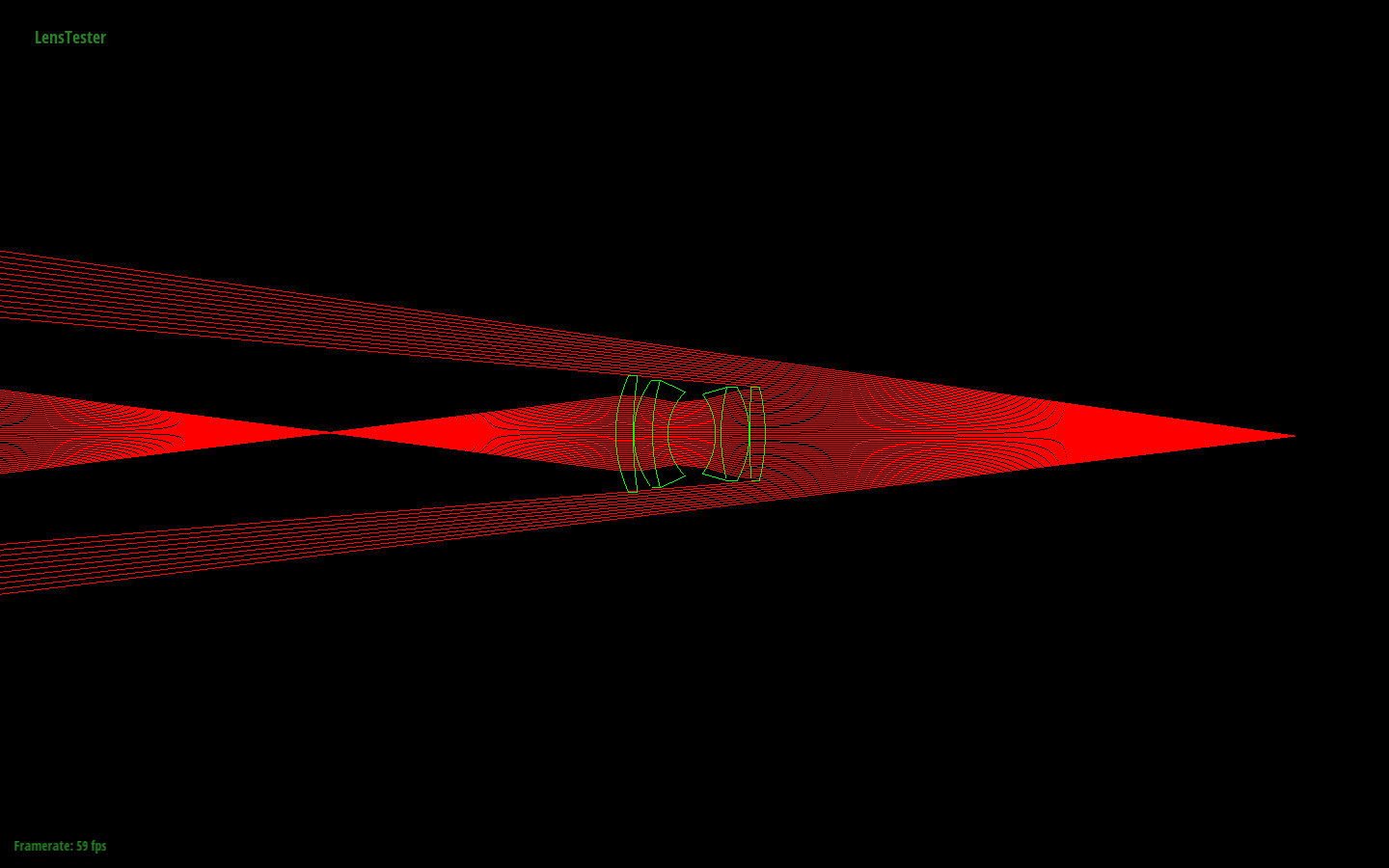
Lens 1. Rays converging at a conjugate point on the left side of the image.
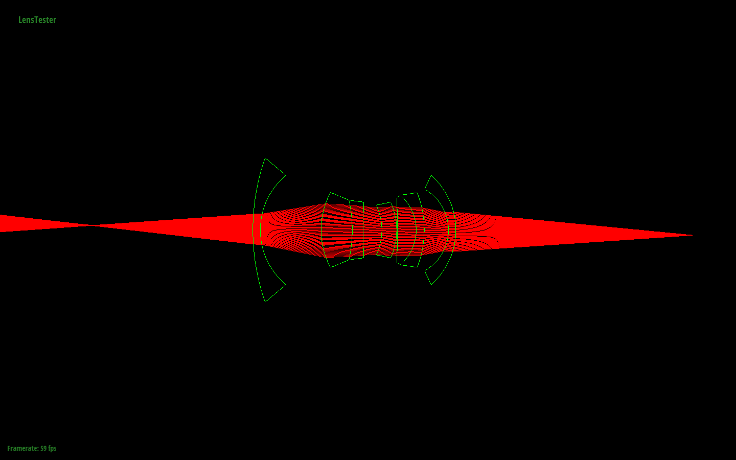
Lens 2. Rays converging at a conjugate point on the left side of the image.
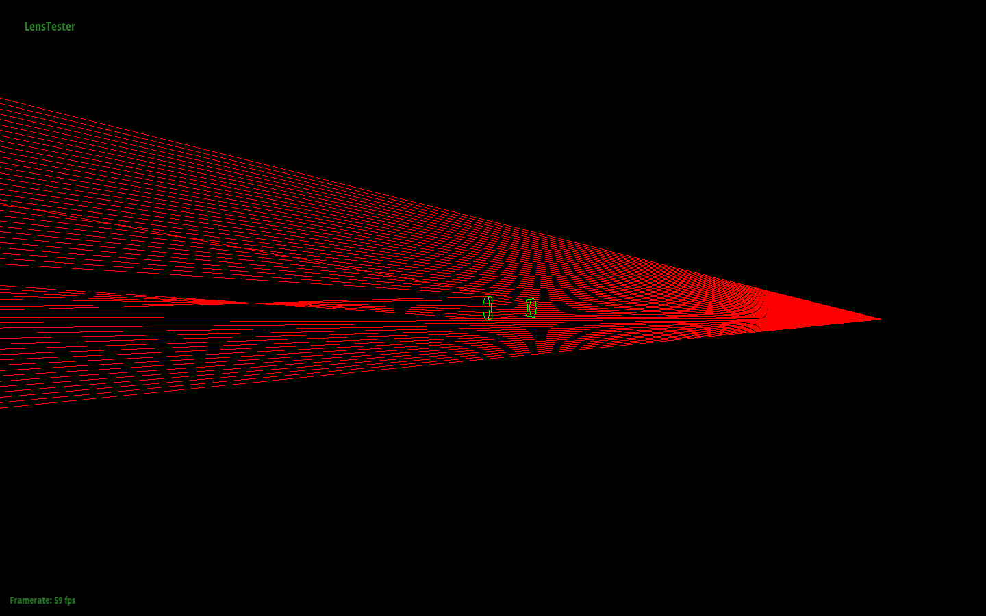
Lens 3. Rays converging at a conjugate point on the left side of the image. This image is zoomed out much more than the others because it is a telephoto lens.
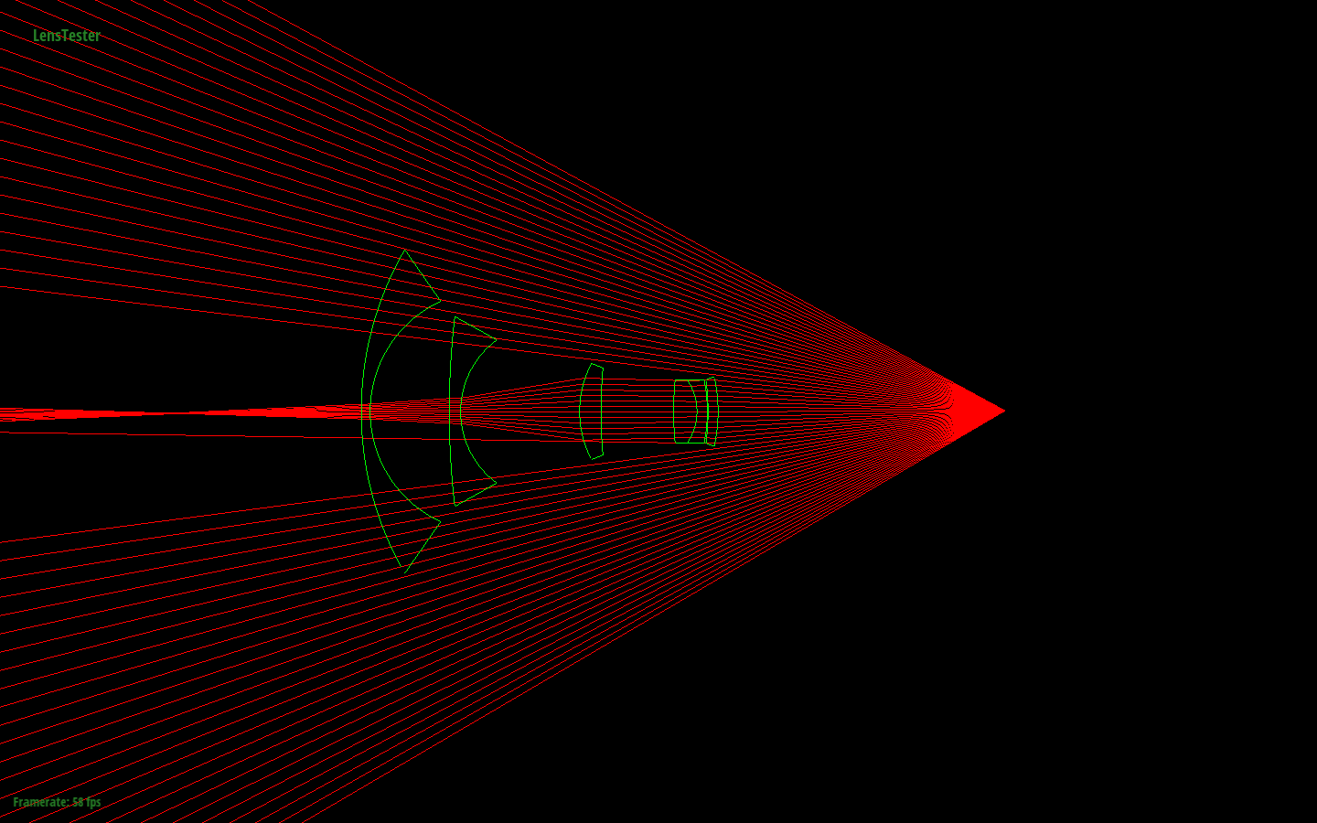
Lens 4. Rays converging at a conjugate point on the left side of the image.
.
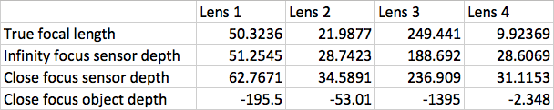
Table of important distances for each lens. All values are in millimeters. All of the depth measurements are relative to the origin of the camera space (Specifically, they are measurements along the z-axis).
.
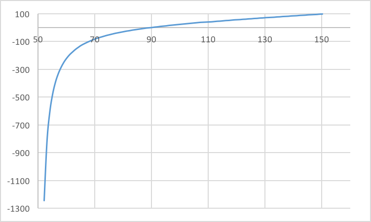
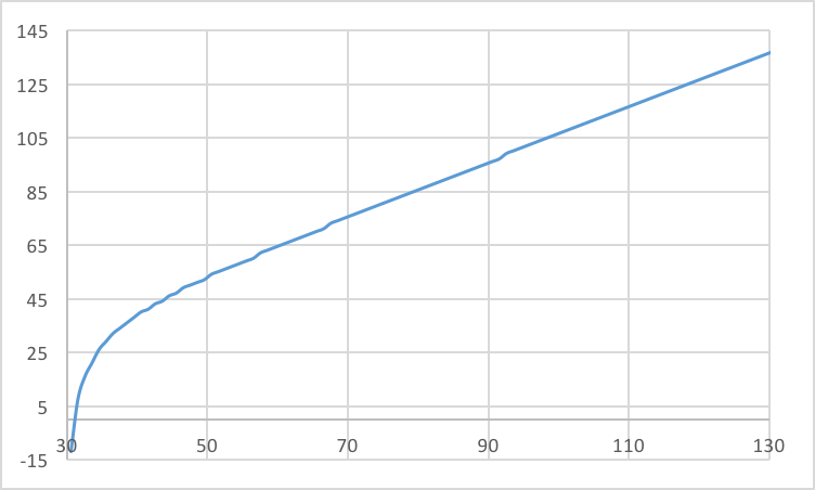
Lens 1. Graph of sensor depth vs. conjugate focus depth. Both the sensor depth (x-axis) and conjugate focus depth (y-axis) are in units of millimeters. This is the D-GAUSS F/2 22deg HFOV lens. It has a fair range of sensor depths (about 52 to 90 mm) for which objects are in near focus (0 to 1 meter away). Beyond that, with the sensor depth below 52 mm, infinity focus occurs as indicated by the asymptote on the left side of the graph.
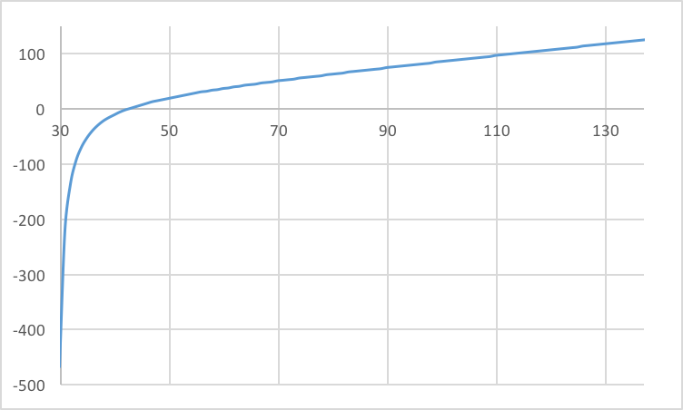
Lens 2. Graph of sensor depth vs. conjugate focus depth. Both the sensor depth (x-axis) and conjugate focus depth (y-axis) are in units of millimeters. This is the Wide-angle Nakamura lens. It has a smaller range of sensor depths than the D-GAUSS (about 30 to 40 mm) for which objects are in near focus. Beyond that, with the sensor depth below 30 mm, infinity focus occurs as indicated by the asymptote on the left side of the graph.
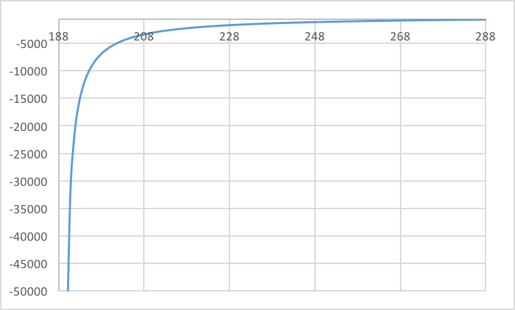
Lens 3. Graph of sensor depth vs. conjugate focus depth. Both the sensor depth (x-axis) and conjugate focus depth (y-axis) are in units of millimeters. As shown by the asymptote on the left side of the graph, with a smaller sensor depth (approaching 190 mm), the conjugate focus depth goes to beyond 50 meters. The conjugate focus is that far away because this graph represents the SIGLER Super achromate telephoto lens. This far away conjugate is also shown by the above lenstester rendering.
Lens 4. Graph of sensor depth vs. conjugate focus depth. Both the sensor depth (x-axis) and conjugate focus depth (y-axis) are in units of millimeters. As shown by the asymptote on the left side of the graph, infinity focus is quickly achieved with a sensor depth below 32 mm. This means that there is only a short range of distances for which objects are in reasonably good near focus, (focus not at infinity). This is because this lens is the Muller fisheye lens. As shown in the convergence image above for lens 4, the conjugate point is very close to the most forward lens.
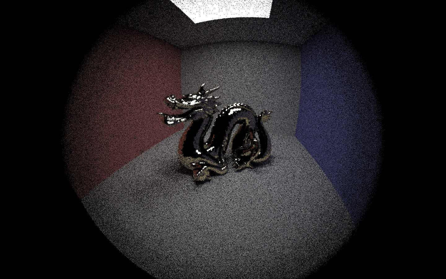
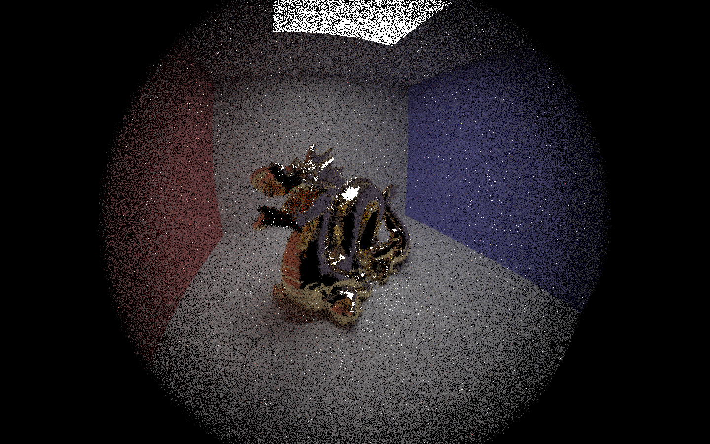
CBdragon.dae at a high rendering quality. Using lens 1 (D-GAUSS F/2 22deg HFOV). The mouth and chest of the dragon are in focus: the metallic surface is shiny and the edges of the object are sharp. The tail end of the dragon is out of focus and blurry: the surface is less shiny and the edges of the object are not distinct. Additionally, the corner of the Cornell box is also out of focus in the distance; the corner is blurry and not sharp, with the white and the blue bleeding together.
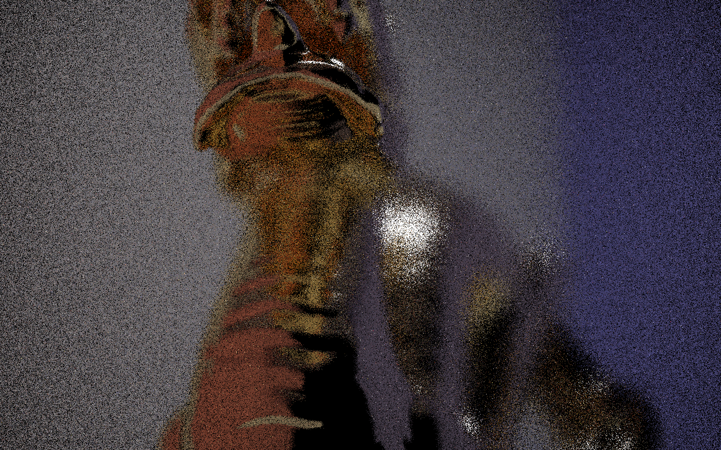
CBdragon.dae at a high rendering quality (Oops, low ray depth). Using lens 4 (Muller 16mm/f4 155.9FOV fisheye lens). The entire dragon here is fairly in focus. However, subjectively the middle curve of the dragon's body appears to be slightly more in focus than the rest of it. Since this is a fish eye lens, a larger hemisphere of the scene is captured compared to the other lenses. Characteristic of this lens type is that the edges of the image (areas with a large angle to the z-axis) are warped and stretched out. This effect can be seen be examining the edges of the Cornell box where the walls meet: these edges turn out to be curved lines rather than straight lines.
Part 2: Contrast-based autofocus
My autofocus algorithm is composed of two parts: a variance-based focus metric and the autofocus heuristic. The algorithm runs on a small cell in the scene to find the sensor depth that best focuses that part of the image.
For my focus metric, I am calculating the RGB variance of the cell. Provided an ImageBuffer of RGB values, the metric first iterates through the buffer and sums up all of the color values in each channel. Then the sums of each color channel is divided by the number of pixels in the ImageBuffer (simply width * height). This gives us the average value of each color channel. Using these mean values, the metric iterates through the ImageBuffer once again, this time summing up the squared differences of each color channel. (For example for the Red channel, vsum_r += (r - x_r) * (r - x_r); where vsum_r is the running sum, r is the red value of the current pixel, and x_r is the previously calculated mean red value.) After iterating through the ImageBuffer, the 3 sums of squared differences of the channels are all added together and divided by the total number of pixels in the ImageBuffer. This value, the Variance of the RGB channels, is returned.
This Variance captures the idea of "focus" in the image cell. This is because, what humans view as an image being in focus is that the image is "sharp." An in-focus image has objects with edges that are clearly visible: the object in the foreground contrasts with the background of the scene. In terms of signal-processing, there are many high-frequency signals in the focused part of the scene. For an out-of-focus image, edges are blurry and objects are indistinct from the background. There are few high-frequency signals in the scene. In terms of my metric, the Variance calculated above captures the idea of quantifying the relative amount of high-frequency signals in the cell. So, if we maximize Variance, we also tend to maximize the number of high-frequency signals, leading to high visual contrast, and therefore the image is in focus.
My autofocus heuristic seeks to maximize the Variance value calculated above. First, the sensor_depth is initialized to be at the len's sensor-depth value infinity_focus. Then the initial step size is set to be the len's sensor-depth values 0.75 * (near_focus - infinity_focus). (The 0.75 was arbitrarily chosen such that the step size is between the two focusing depths: this way the step size is neither too big or too small.) Two variables record the maximum variance achieved and the depth at which that maximum variance was achieved. Then while the step size is greater than 0.005 (millimeters), we loop: (I) one step size is added to sensor_depth; (IIA) if the variance is increased in the cell, record the current state and maximum values, and continue the loop to step again; (IIB) otherwise if the variance is decreased after stepping, keep the current sensor_depth step, divide the step size by negative two, and loop to step again using the new step size. My algorithm divides the step size by negative two in order to (1) decrease the step size and (2) reverse the direction of stepping. My justification for keeping the "missteps," when the sensor_depth is overstepped and the variance decreases, and reversing directions, is to try to avoid local maxima "traps" in variances.^* The loop breaks when the step size is below 0.005 mm. Then, the sensor_depth is finally assigned to be the depth at which the maximum variance was recorded. The cell is then in focus.
^* My algorithm weakly protects against the local maxima when trying to find the global maximum in variance. When an overstep occurs, the variance is less than before the step. However, the sensor_depth values is kept, and we instead step backwards. If the global maximum was jumped over, then variance should increase once again while stepping backwards and we eventually reach the global maximum as intended. If a local maximum was jumped over, stepping backwards may indicate another decrease in variance, in which case direction is reversed again and we step forwards to increasing variance. Hopefully, the new stepping forwards will lead to the global maximum. It is possible to keep jumping over local maxima, but it is unlikely due to the continually decreasing step size.
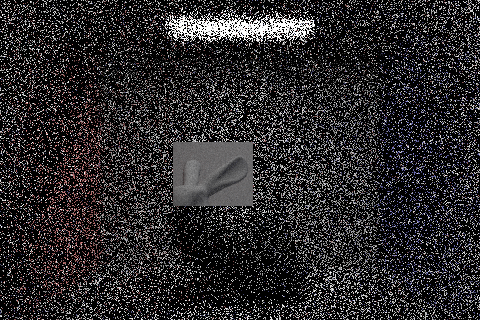
An image with autofocusing done with respect to the ears of the bunny. The shadows and the ambient occlusion around the bunny ears make this a good place to test the autofocus algorithm. The ears are high contrast elements.
Graph of my autofocus algorithm running on the above cell. The x-axis of this graph is sensor depth (millimeters) and the y-axis of this graph is variance (a unitless value representing the total variance of RGB values in the cell). A global maximum can be seen at 54.692 mm with a variance of 787.177. This is the sensor depth which produced the cell in the above image. (This graph includes the variance values of missteps, when the global maximum variance is overstepped.)
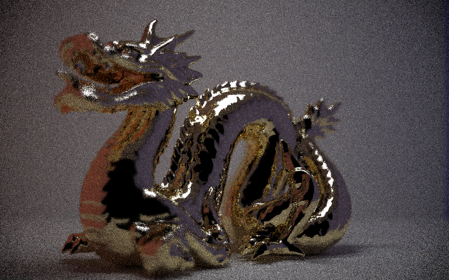
Lens 1, focusing on the middle of the middle bump of the dragon. The bright specular shine of the metal contrasts well with the dark reflection of the open end of the Cornell box. The head of the dragon is out of focus, particularly towards the front of the mouth. Similarly, the tip of the tail is out of focus.
Lens 2, focusing on the top of the middle bump of the dragon. In particular, the backside of the middle bump turned out to be particularly in focus. Perhaps enough light reflected off the bottom curves of the dragon and hit that backside to cause the algorithm to choose this sensor depth. Notably, because this is a wide angle lens, both the red and the blue wall can be seen! Like the above image, the mouth and tail of the dragon are out of focus.
Lens 3, focusing on the horns on the back of the dragon's head. Because this was a telephoto lens, the image had to be taken zoomed far away from the scene. As a result, there is little relative (camera z-position) distance between the surfaces of the dragon. The focusing was done on the dragon's horns, but the rest of the dragon is fairly in focus as well. Additionally, because of the small capturing angle of the lens, only the back wall is shown here -- in contrast to seeing both walls in the above wide angle lens image.
Lens 4, focusing on the middle of the middle bump of the dragon. The edges of the 'scales' appear fairly well defined. There is high contrast between that middle dark spot and the bright specular reflection above it. As noted in the previous parts, the edges of the lens warp the image. Because the fisheye lens captures a large hemisphere of the scene, the center of the image appears fairly realstic in proportions while the edges are out of proportion. The edges of the Cornell box are curved rather than straight.
Part 3: Faster contrast-based autofocus (Extra credit)
As explained in Part 2, my original algorithm weakly protects against falling into local minima traps. In contrast to the naive approach of not keeping oversteps and never reversing directions in stepping, my algorithm tends to find better quality focusing depths. The outcome tends to be better using about the same amount of time.
For creating the following two images, I had modified my algorithm to the naive approach. I am focusing on the top of the middle bump of the dragon:
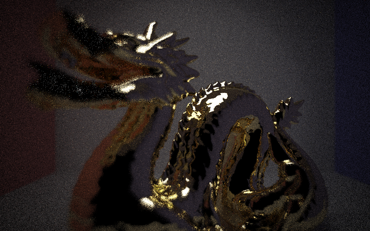
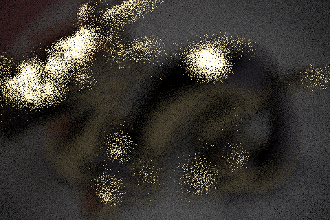
The naive algorithm. It seems that the specular shine of the metal produced a large enough variance to trap the sensor_depth step-based traversal. As a result, the image is blurry except for the large splotches of reflected light.
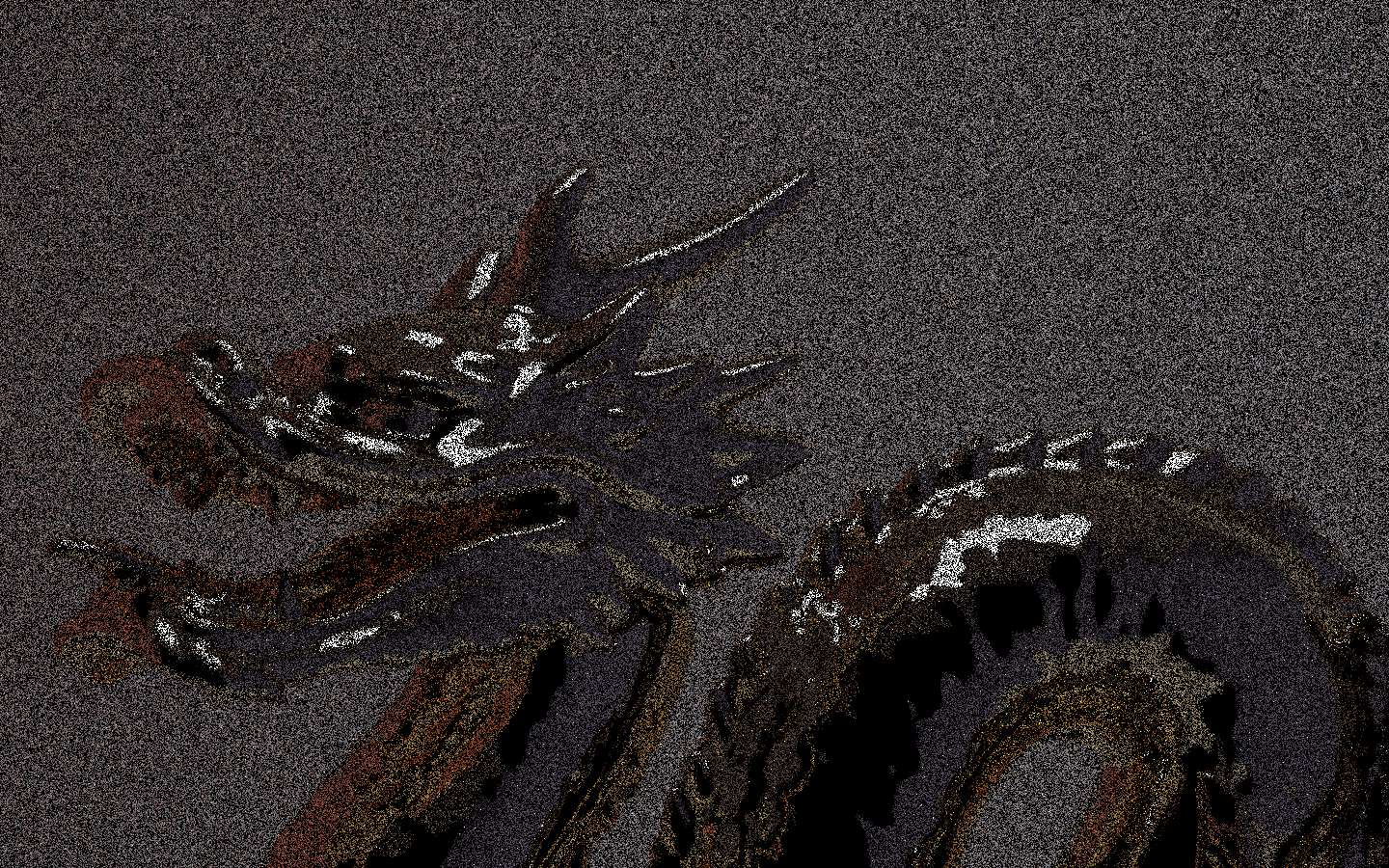
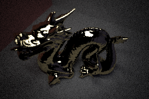
The algorithm which does backsteps. At this angle, my original algorithm managed to avoid the local maxima from the specular shiny metal. Unfortunately, the top of the tail bump is not fully in focus. The middle section further down on the tail seems to have slightly sharper edges. (This image is rendered at the same zoom level as the above, the sensor_depth makes a large difference.