CS194-26 | Frequencies and Gradients
Allen Zeng, CS194-26-aec
Part 1 - Frequency Domain Processing
1.1 - Sharpening Images
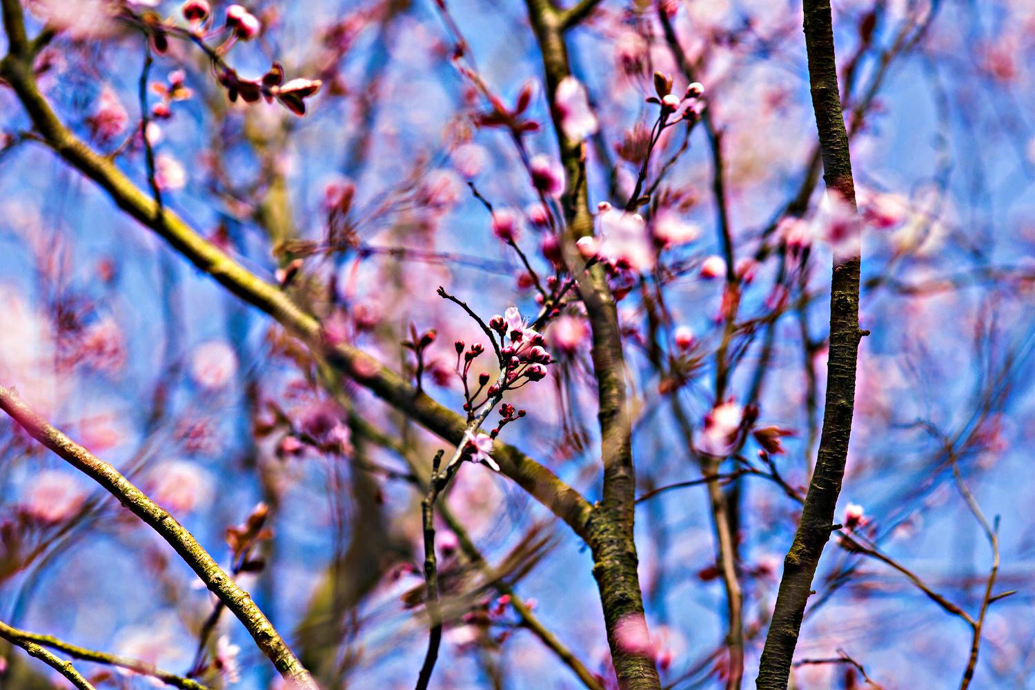
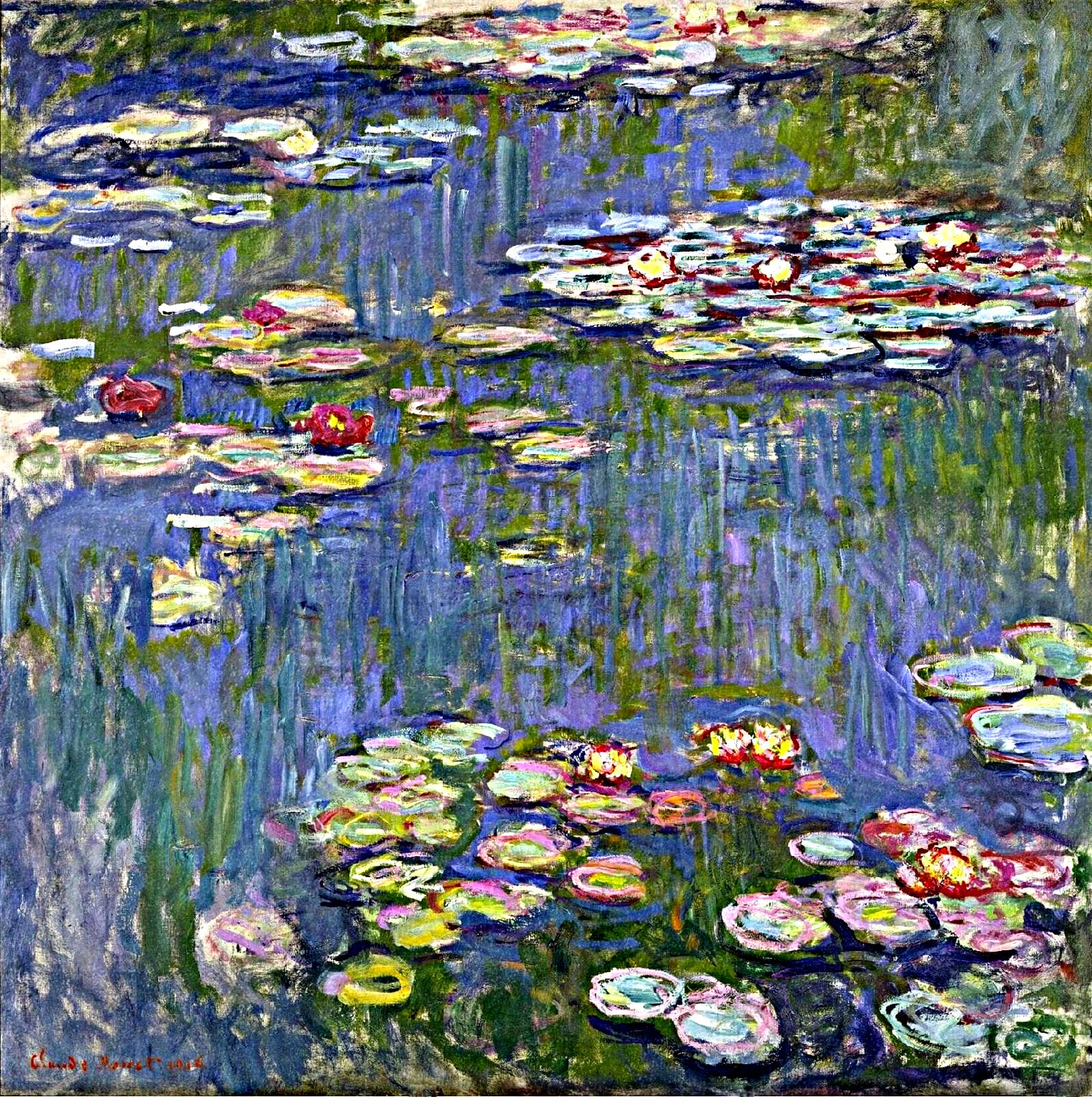
Edges in an image are represented by high frequency changes among pixels. So to sharpen images, we can increase the magnitudes of the higher frequencies in the frequency domain. One way to approach that goal is through the "unsharp masking" technique.
For the unsharp masking technique, first we obtain the lower frequency signals in an image by applying a Gaussian blur to the entire image. A Gaussian blur effectively removes higher frequencies from an image. Then we subtract the blurred image from the original to obtain the Laplacian of the image. The Laplacian contains the difference in signals of the original and the blurred image, which are the high frequency signals that were removed from the blurring process. Finally, the Laplacian is positively scaled and added back onto the original image. This results in an image where the higher frequencies are boosted in magnitude.
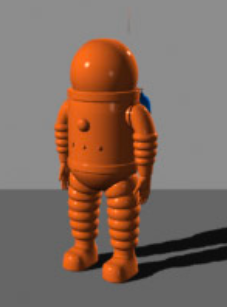
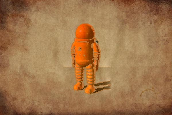
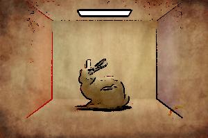
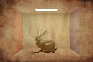
| Before | After |
|---|---|
Flower, Original
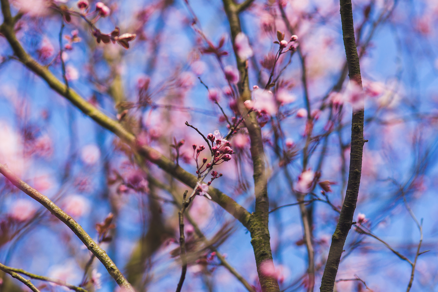
|
Flower, Sharpened
|
Water Lilies, Monet, Original
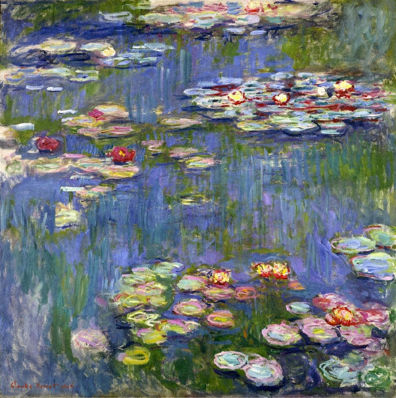
|
Water Lilies, Monet, Sharpened
|
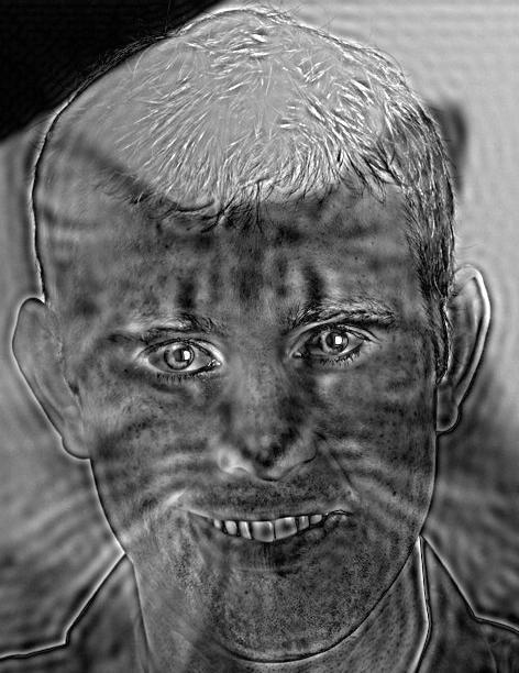
1.2.1 - Hybrid Images
Images contain a wide range of frequencies. From a long distance, humans tend to perceive low frequency signals in an image better. And from a short distance, humans tend to perceive high frequency signals in an image better.
By combining the low frequency components of one image and the high frequency components of another image, we can create a hybrid image. The hybrid image will look differently at different distances. There are many ways to implement these hybrid images, such as using different filtering techniques.
Here, I use the Gaussian blurring technique to process the images. The low frequencies are obtained directly by Gaussian blurring, as in part 1.1. The high frequencies are obtained by subtracting the Gaussian blurred image from the original, also as in part 1.1. The two resulting images are averaged to create the hybrid.
Try looking at the following images close to the screen (seeing high frequencies), and then far away from the screen (seeing low frequencies). Using different zoom levels on the webpage work as well.
| Low Frequencies From: | High Frequencies From: | Hybrid Image |
|---|---|---|
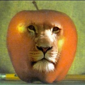
Nutmeg
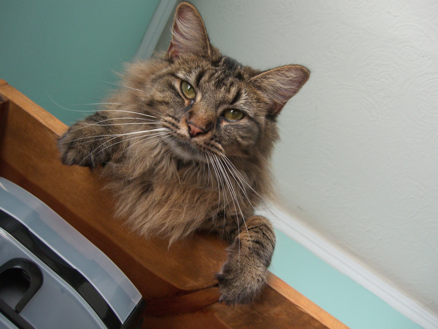
|
Derek
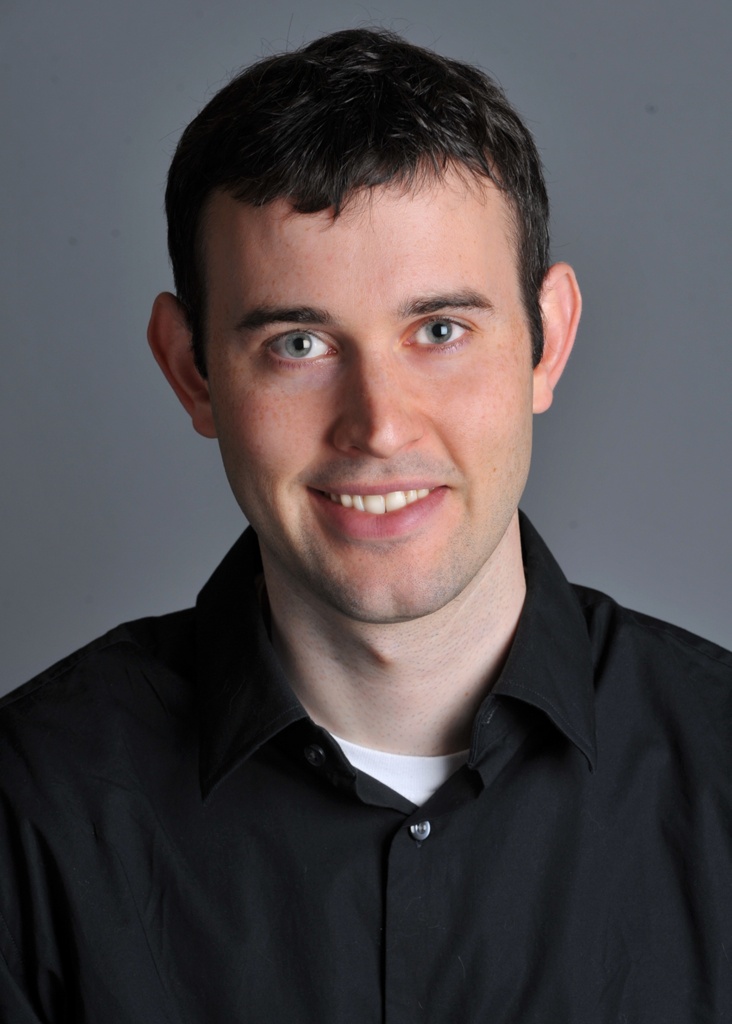
|
Nutrek
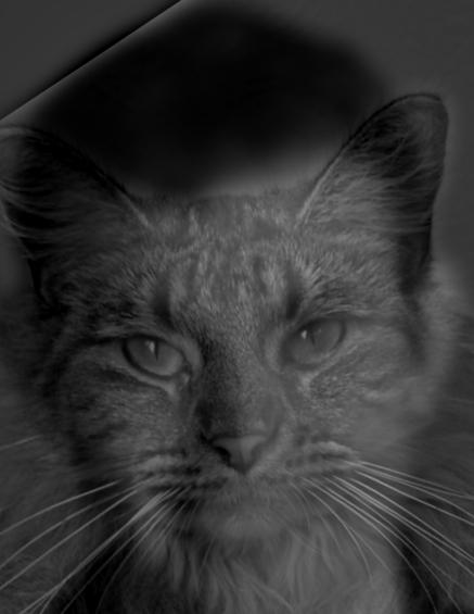
|
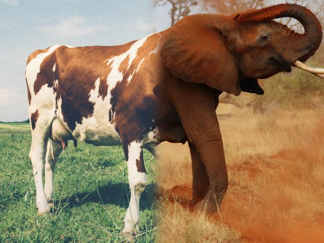
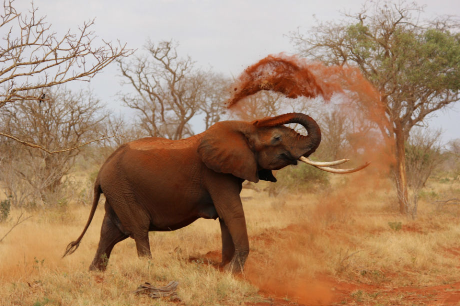
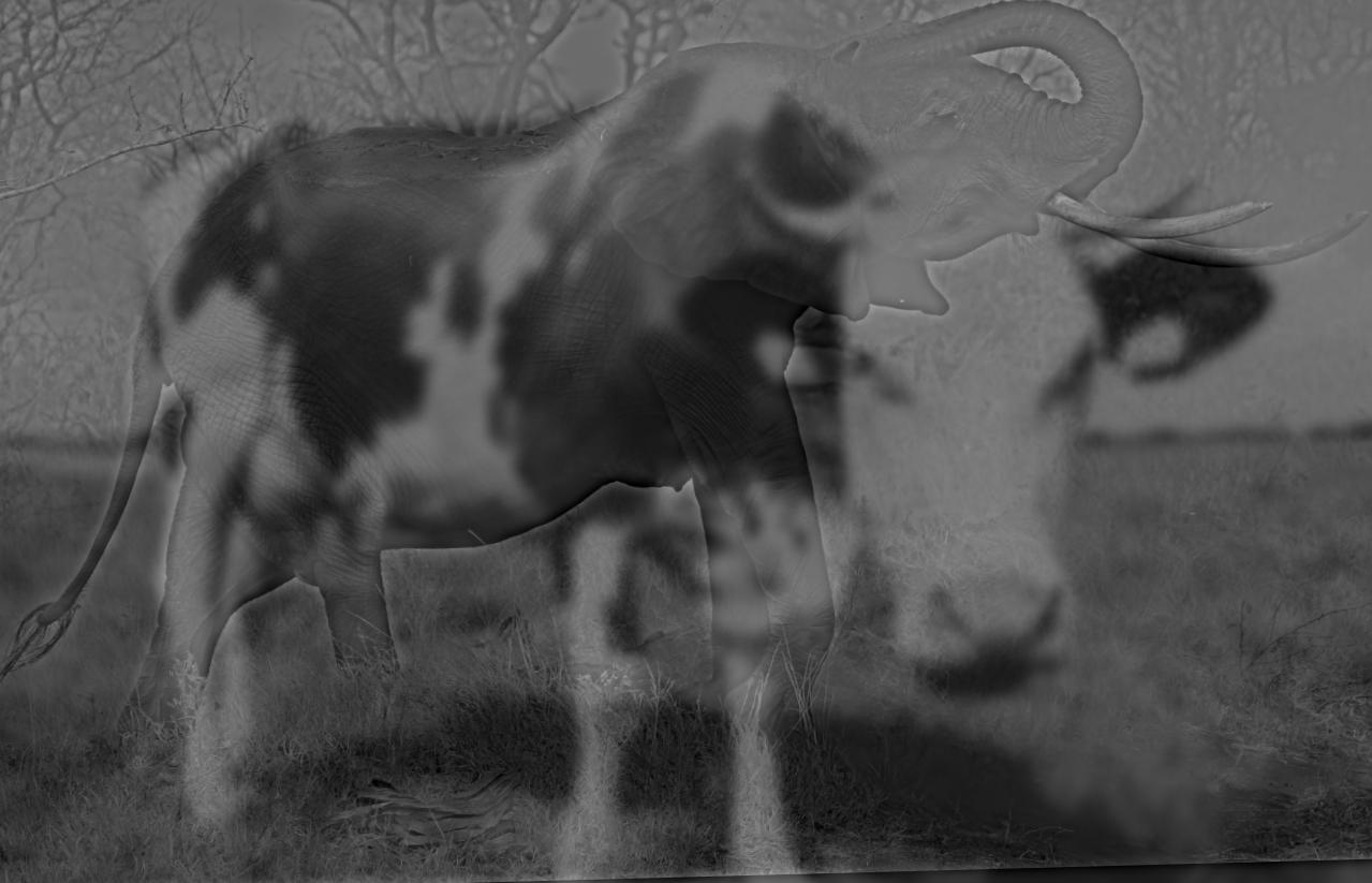
Cow
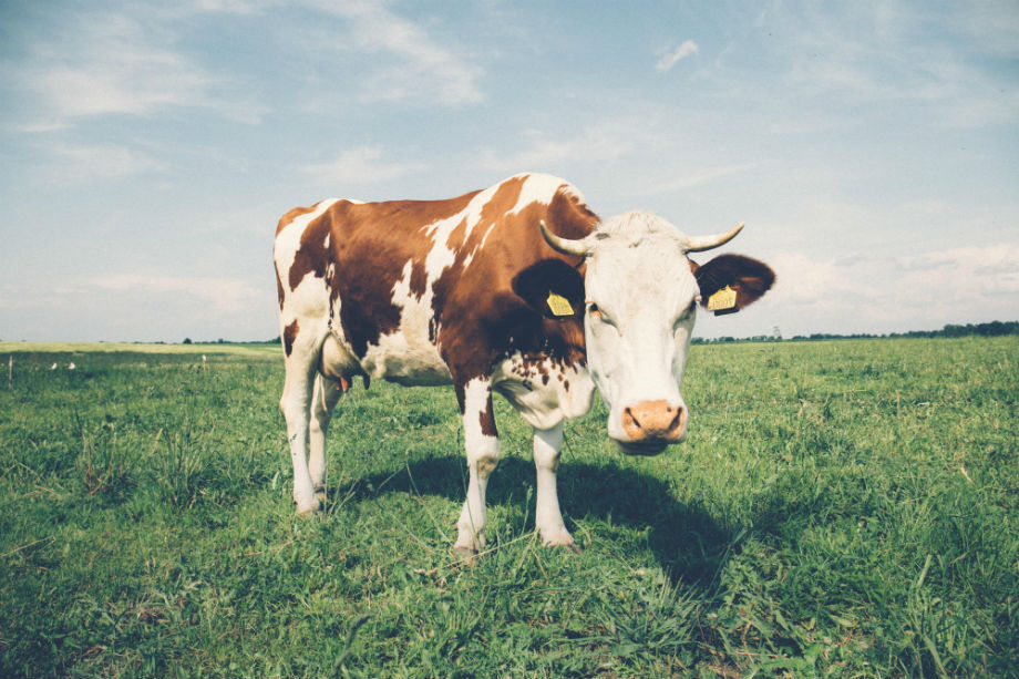
|
Elephant
|
Cophant
|
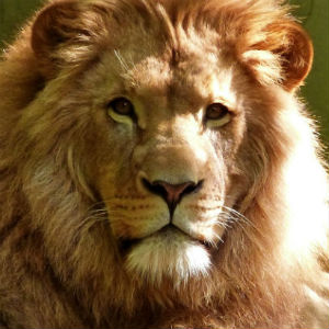
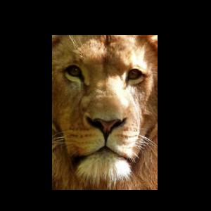
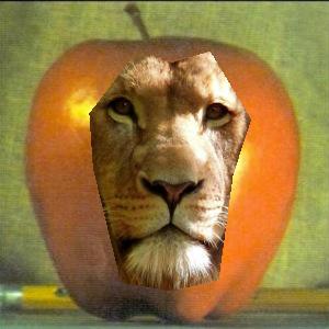
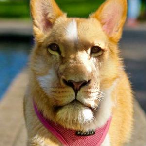
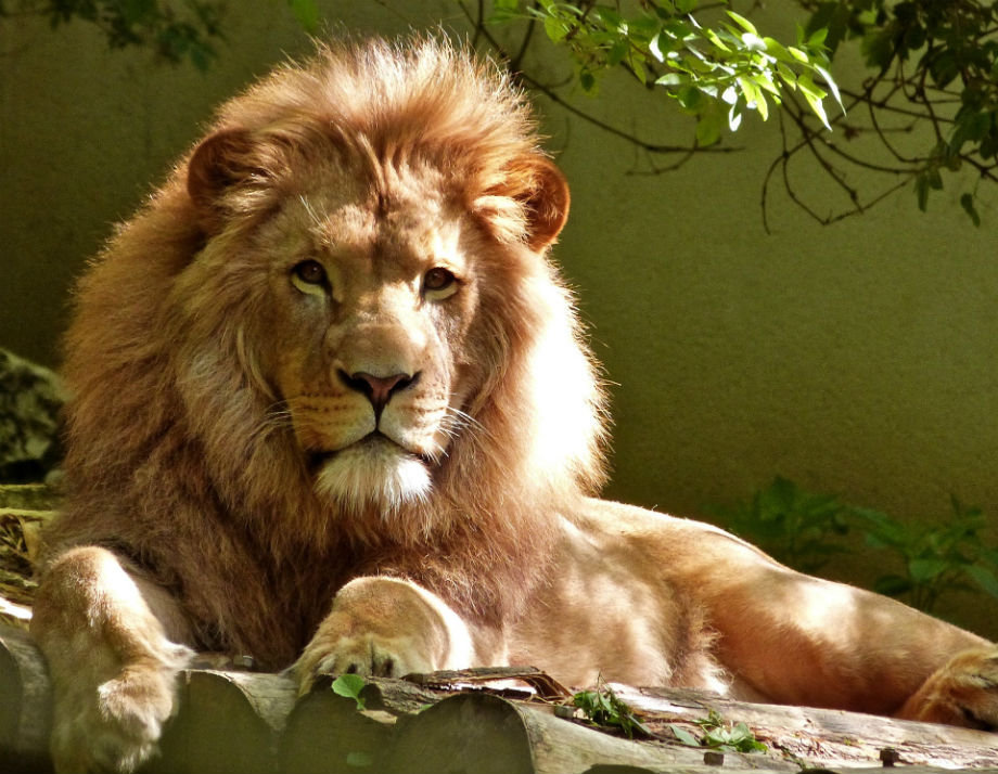
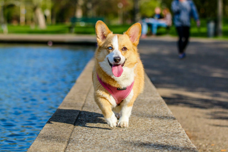
Lion
|
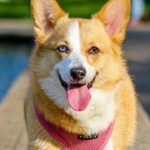
Corgi
|
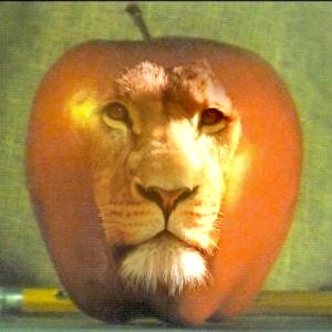
Liorgi
|
1.2.2 - Analysis of Hybrid Images
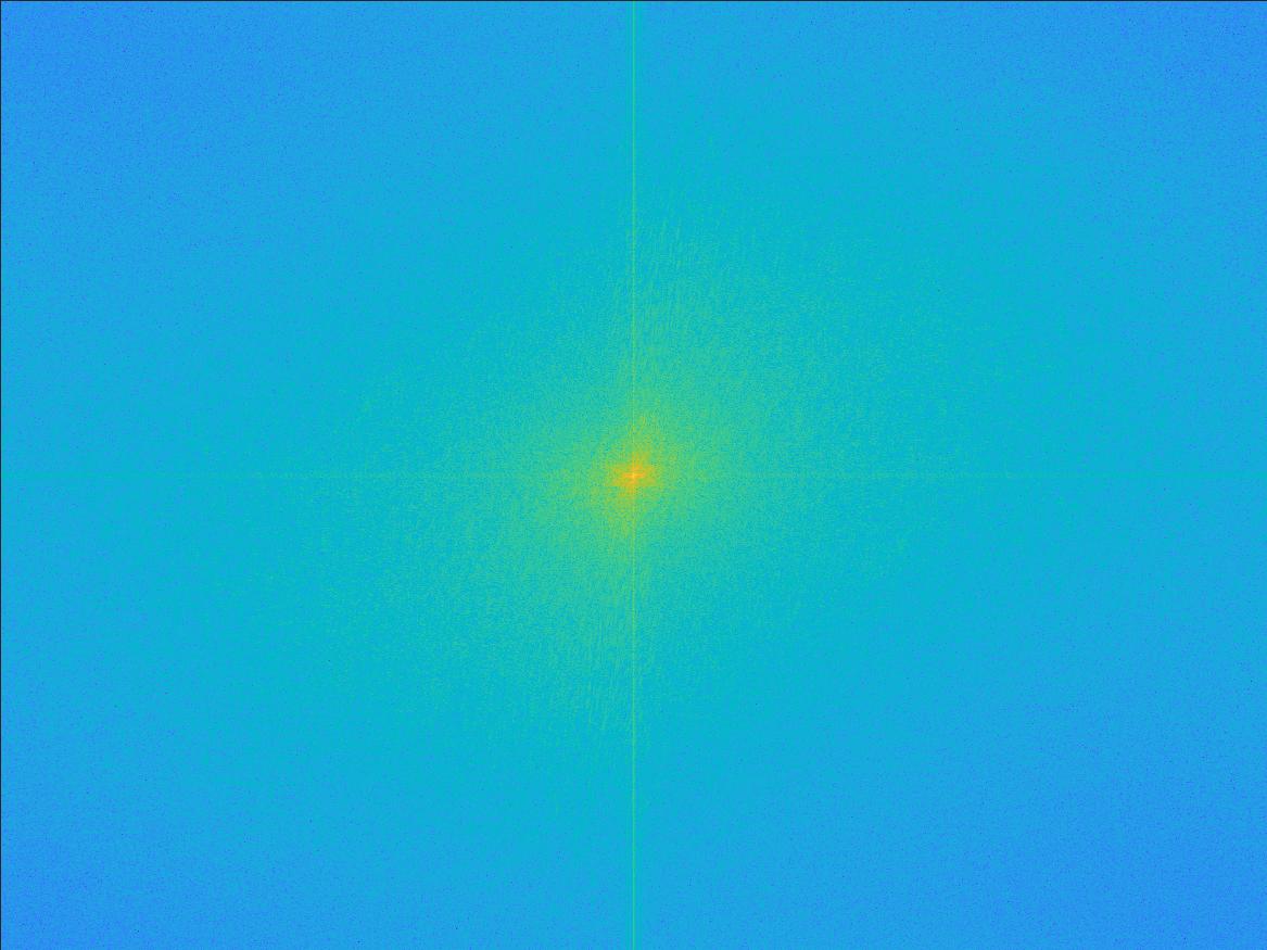
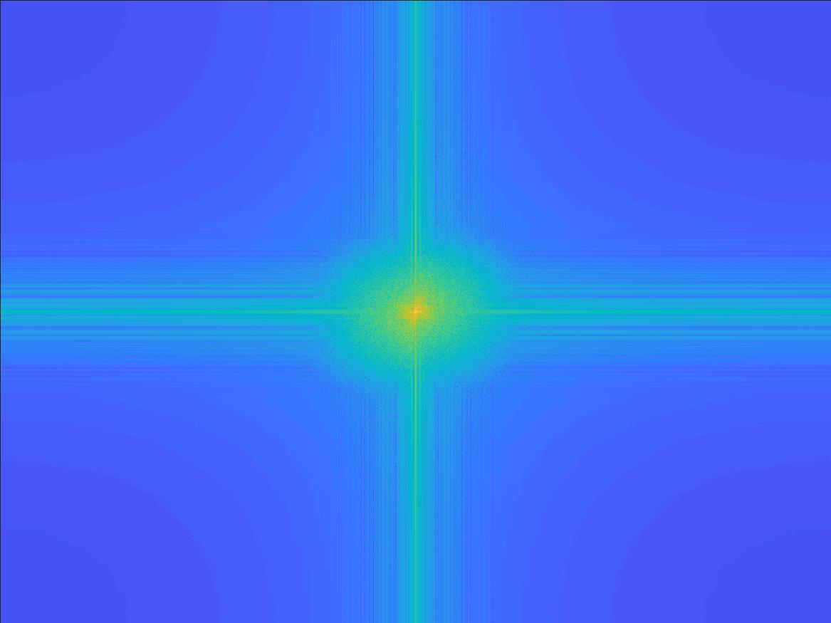
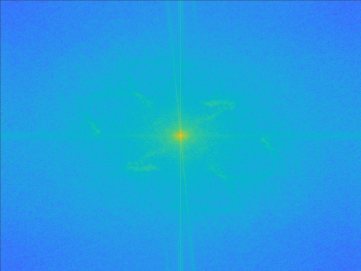
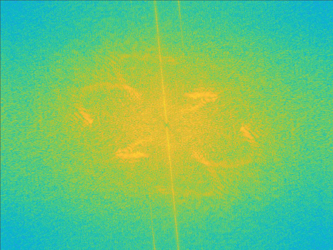
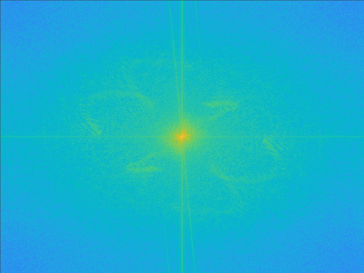
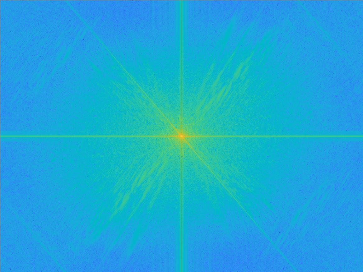
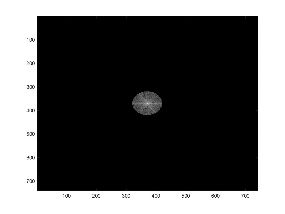
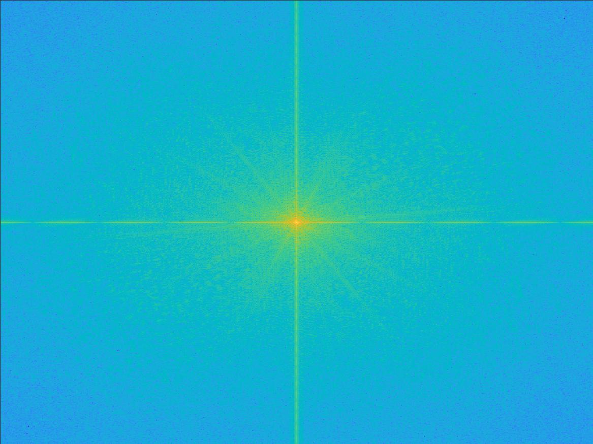
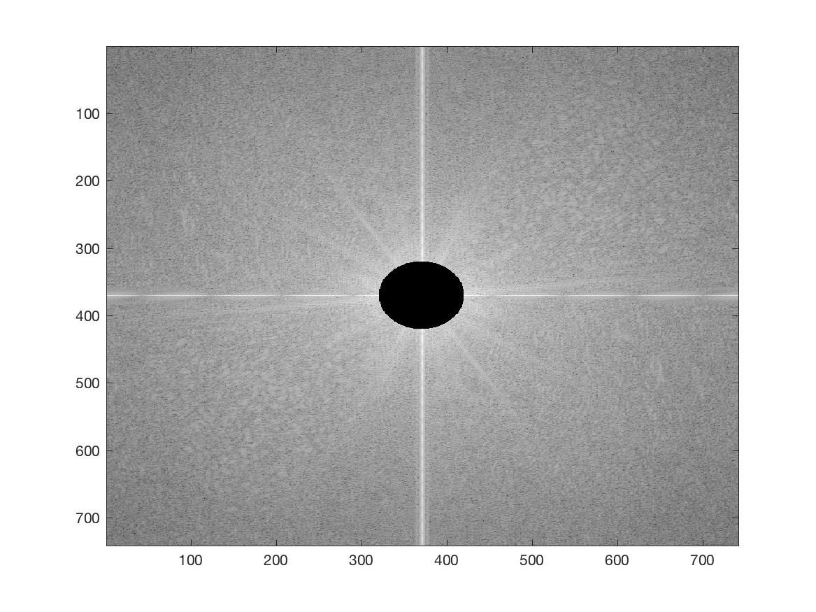
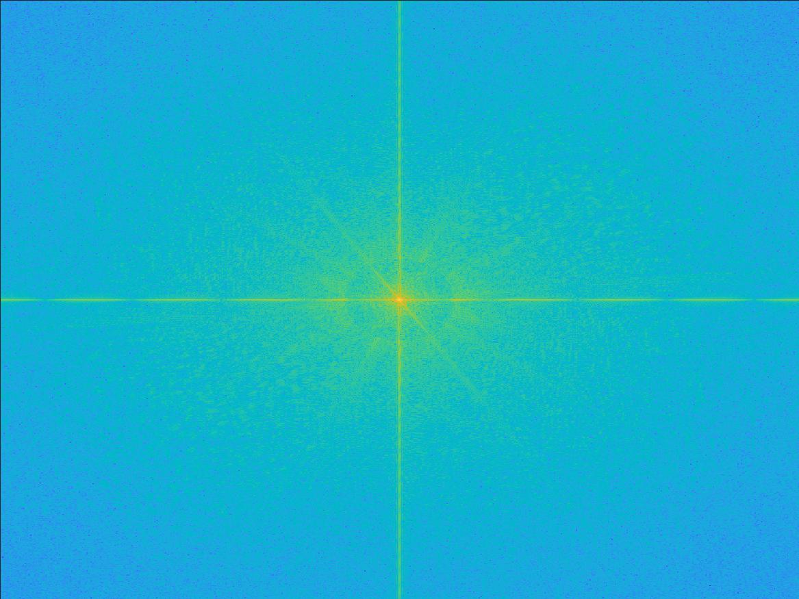
For the lion-corgi hybrid image, the following is a frequency-domain analysis of the hybridization process. The plots are log absolute magnitudes of 0-centered 2D FFT images.
In MATLAB code: imagesc(log(abs(fftshift(fft2(gray_image)))))
The 2nd transform, containing mostly low frequencies, is characterized by the bright vertical and horizontal lines intersecting at the center. The 4th transform, containing mostly high frequencies, is charaterized by the bright sqiggles away from the center. Its center is a low-value teal color. The 5th transform, being the hybrid image, has both the bright vertical and horizontal lines, and the squiggles.
| Lion
|
Corgi
|
Liorgi
|
||
Transform of Original
|
Transform of Low Frequency Image
|
Transform of Original
|
Transform of High Frequency Image
|
Transform of Hybrid Image
|
Failure Case
As mentioned above, there are multiple ways to implement the combining of low and high frequencies. Instead of applying Gaussian blur in the image domain to extract frequencies, I also attempted to apply box filters in the frequency domain.
Convolving with a Gaussian function in the image domain is equivalent to multiplying by a different Gaussian function in the frequency domain. But, multiplying by a box function in the frequency domain is equivalent to convolving with a sinc function in the image domain. Due to the fact that a box filter has discrete edges/is not continuous, the change in frequencies are no longer smooth like in the Gaussian case. This means the resulting hybrid image has jarring visual artifacts, and is not as pleasant to look at. There is no natural "transition" going from perceiving one image to the other one, they both appear overlapped.
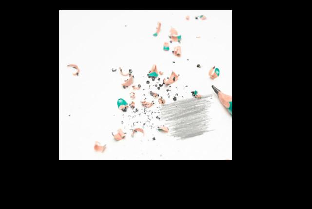
| Nutmeg
|
Derek
|
Nutrek
|
||
Transform of Original
|
Transform of Low Frequency Image
|
Transform of Original
|
Transform of High Frequency Image
|
Transform of Hybrid Image
|
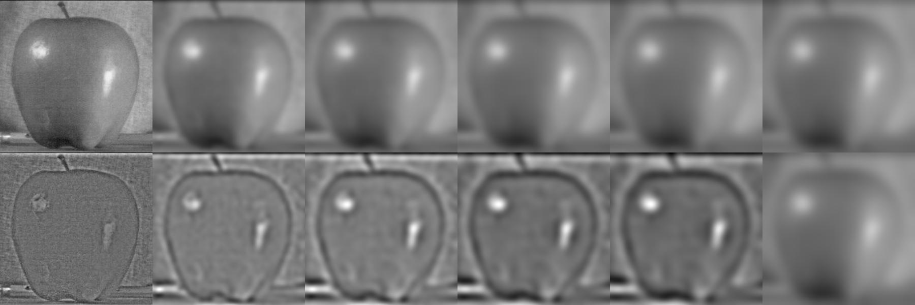
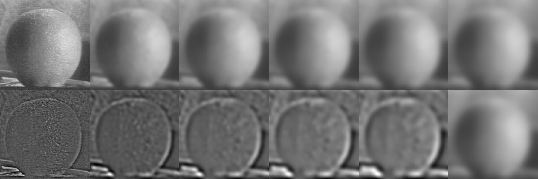
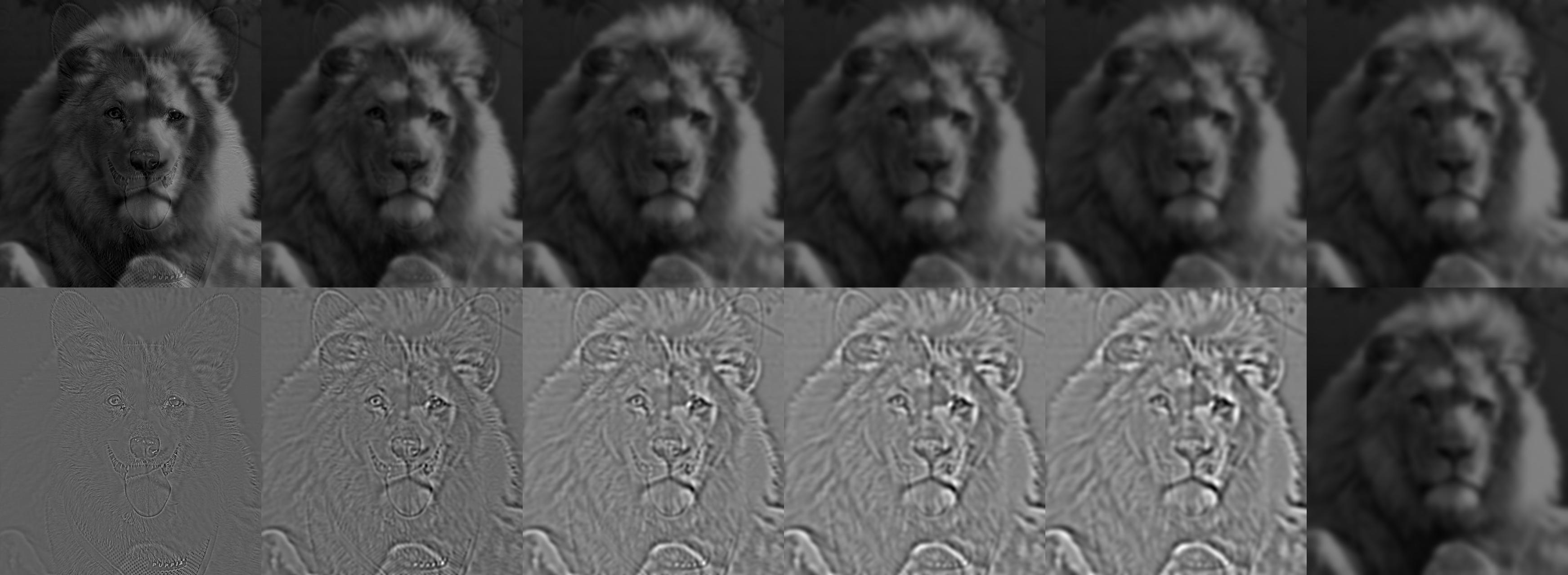
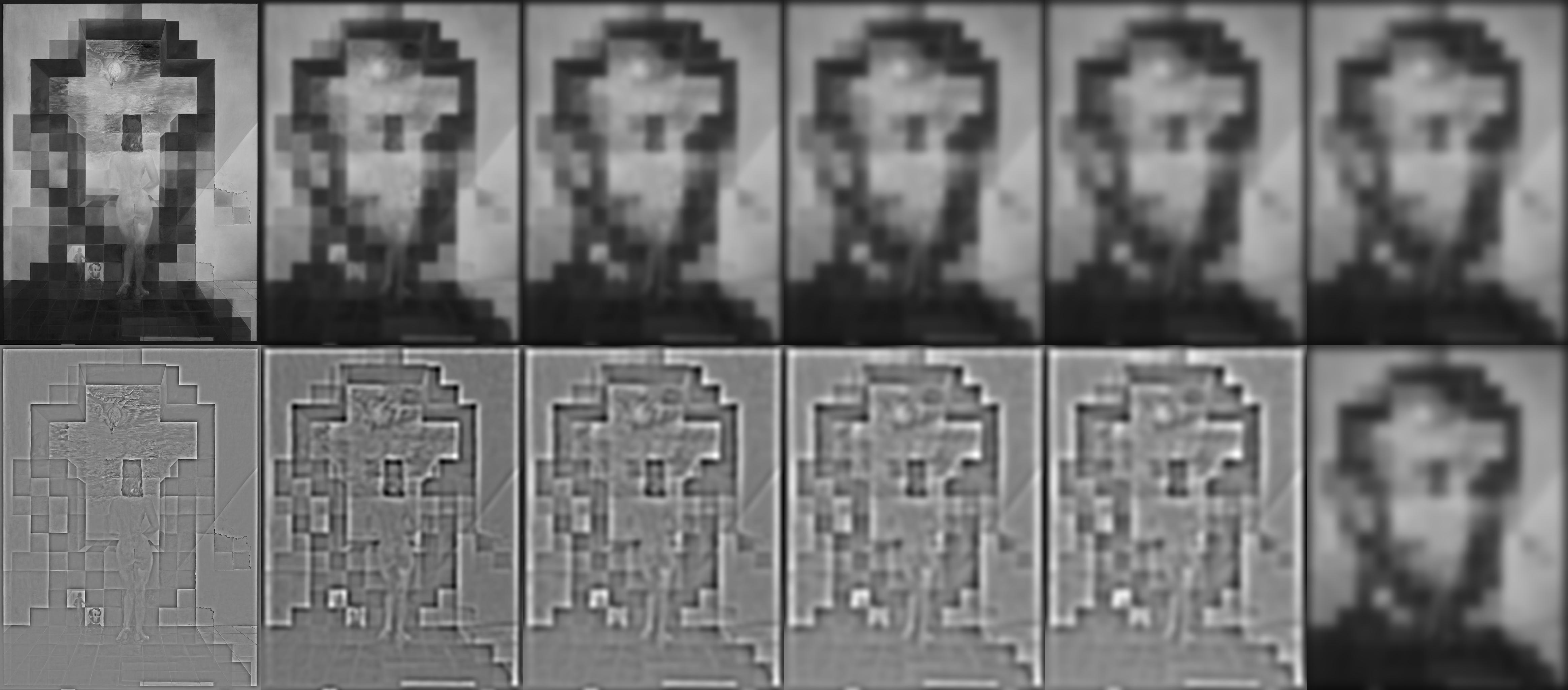
1.3 - Gaussian and Laplacian Stacks
In a Gaussian stack, each image is the previous image with a Gaussian blur applied.
In a Laplacian stack, each image is the difference between two images. In my stack, an image in the Laplacian stack is the difference between the Gaussian stack image directly above it, and the Gaussian stack image up and to the right of it. The last Laplacian image in my stack is just the final Gaussian image.
Essentially, the Laplacian stack captures the loss in frequencies as the Gaussian blur is applied at each level of the Gaussian stack.
The following images have the Gaussian stacks lined up on the top row, and the Laplacian stacks lined up on the bottom row. Please click-to-enlarge or zoom in on the following images.
For the Liorgi stacks, notice that the leftmost Laplacians looks like a corgi, and then the rightmost Laplacians look like a lion. The Gaussian levels simulate viewing the hybrid image at different distances. For the Gala stacks, the left side looks like Gala contemplating the mediterranean sea out of a window. The right side looks like Abraham Lincoln. Again, the Gaussian levels simulate viewing the hybrid image at different distances.
| Gaussian stack images on top, Laplacian stack images on bottom | ||||||||||||||||||||||||||||||||||||||||||||||||||||||||||||||||||||||||||||||||||||||||||
|---|---|---|---|---|---|---|---|---|---|---|---|---|---|---|---|---|---|---|---|---|---|---|---|---|---|---|---|---|---|---|---|---|---|---|---|---|---|---|---|---|---|---|---|---|---|---|---|---|---|---|---|---|---|---|---|---|---|---|---|---|---|---|---|---|---|---|---|---|---|---|---|---|---|---|---|---|---|---|---|---|---|---|---|---|---|---|---|---|---|---|
Liorgi Stacks
|
||||||||||||||||||||||||||||||||||||||||||||||||||||||||||||||||||||||||||||||||||||||||||
Gala Contemplating the Mediterranean Sea which at Twenty Meters Becomes the Portrait of Abraham Lincoln, Dali
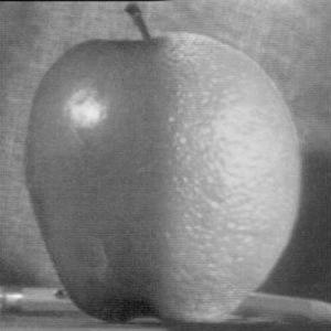
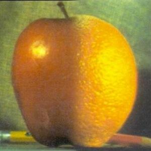
1.4.1 - Multiresolution Blending
We can blend different images together using Gaussian and Laplacian stacks. Since Laplacian stacks represent different buckets of frequencies, we can blend those buckets individually. Then adding the blended bucket-images together will result in an overall blended image. Using a mask, this technique works for irregular shapes in images.
1.4.1 - Multiresolution Blending Results, in Color!In order to blend colored images, the technique described above was applied to each RGB color channel separately.
This technique works best when the backgrounds are similar; or when one image provides the entirety of a background, and the other is overlayed on top.
Part 2 - Gradient Domain ProcessingThe gradients of an image describe how pixel intensities change from pixel to pixel. As images are two dimensional, gradients exist in both vertical and horizontal directions. By working in the gradient domain, we can blend pictures together while retaining their important features and individual textures. Part 2.1 - Toy Problem
Gradients describe how an image change from pixel to pixel. Given an image, we can extract all of the gradient information from it. Then given a single seed pixel, say a corner pixel, we can fully reconstruct an image. If the seed pixel is the same as the pixel in the original image, the reconstruction is extremely small error compared to the original. That is, they are essentially the same image. If the seed pixel is different, then the resulting picture ends up being colored differently. But the textures and figures within the image remain visible. In a way, it can be said that human perception focuses gradients, changes in an image, rather than just seeing colors.
Part 2.2.1 - Poisson Blending
Using the concept of gradients, we can blend together two images while keeping their textures apparent. The color of the input images could end up changing, but the end result is that there are few noticeable artifacts in the output.
Part 2.2.2 - Poisson Blending Results
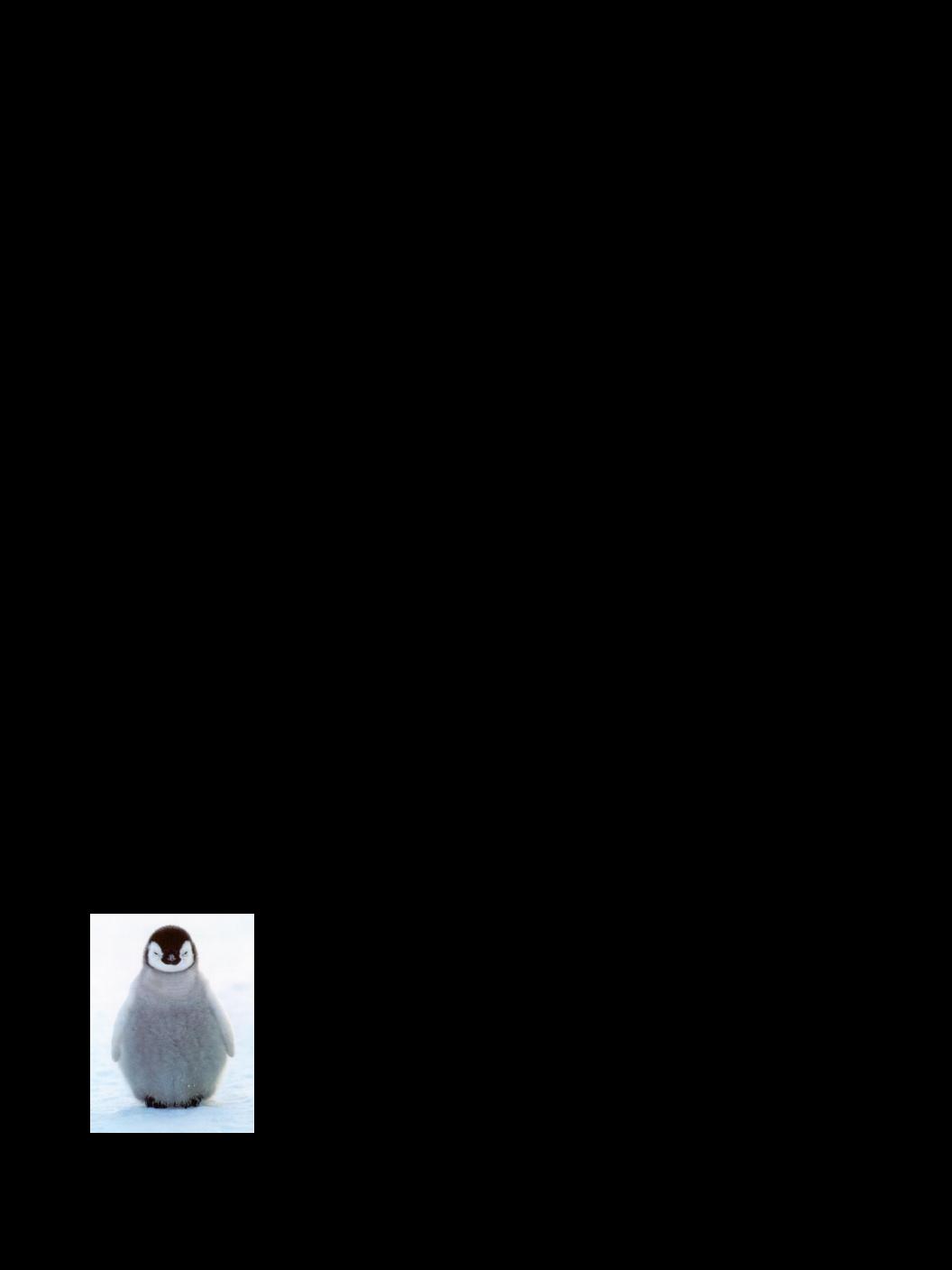
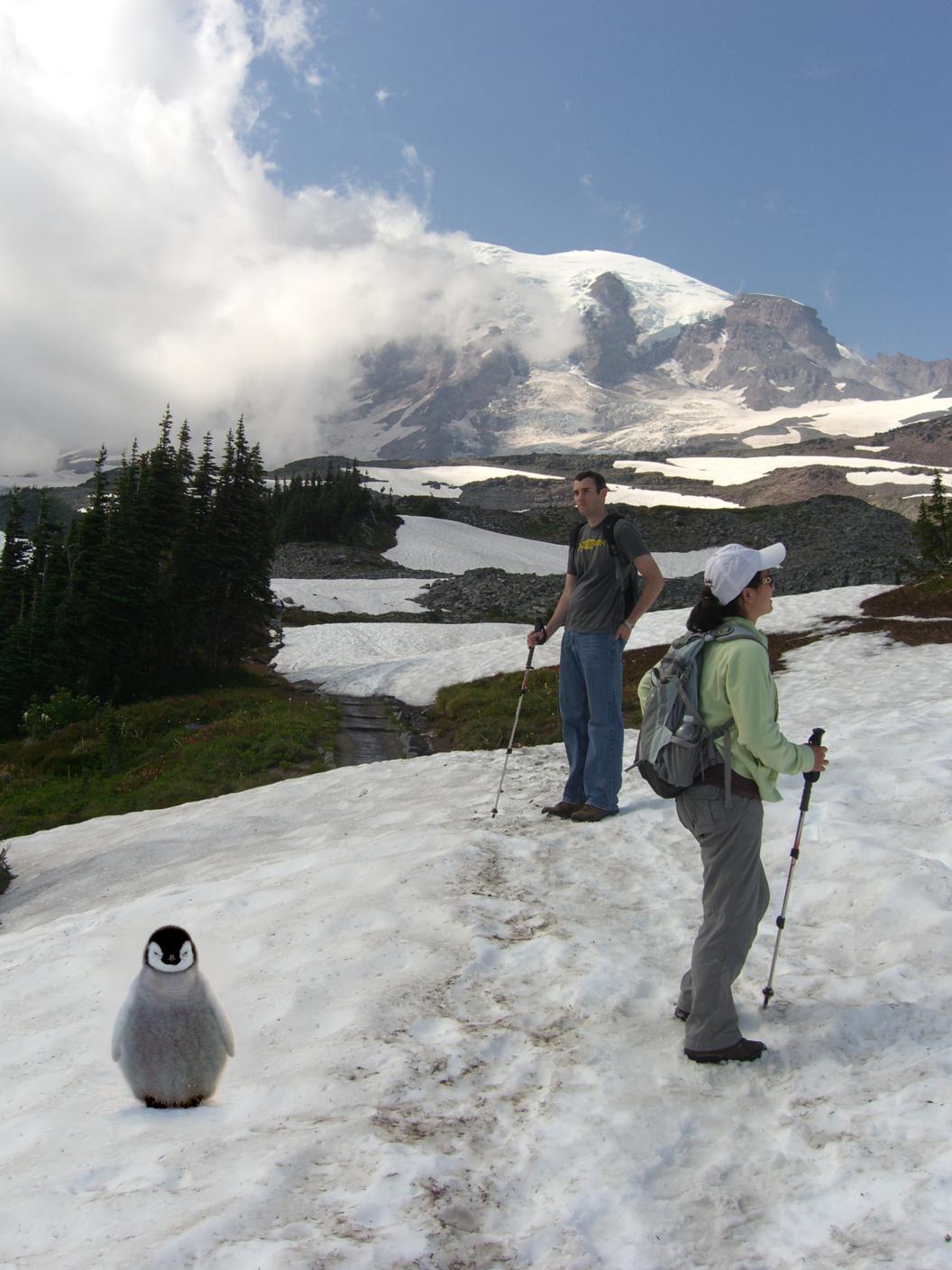
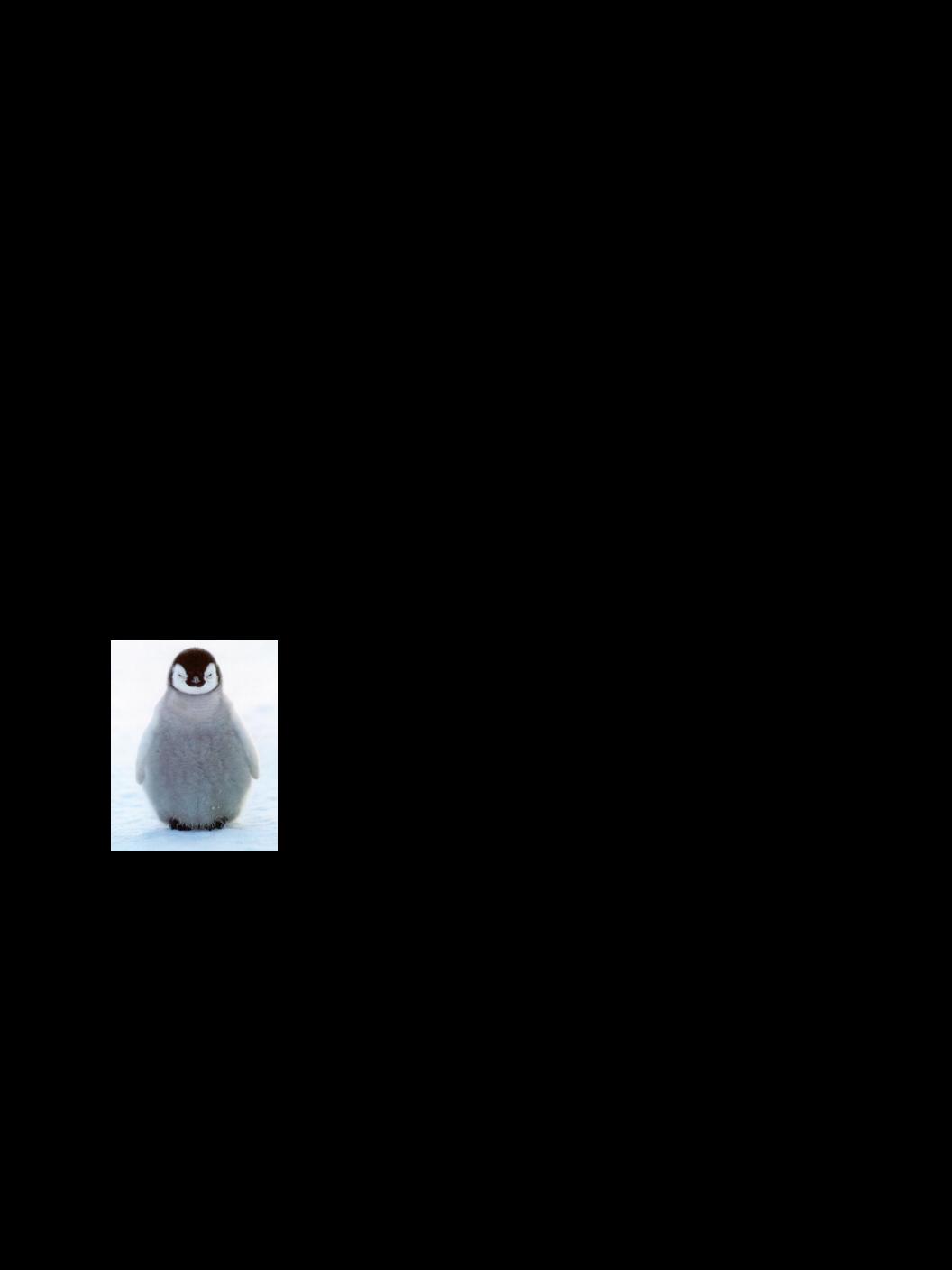
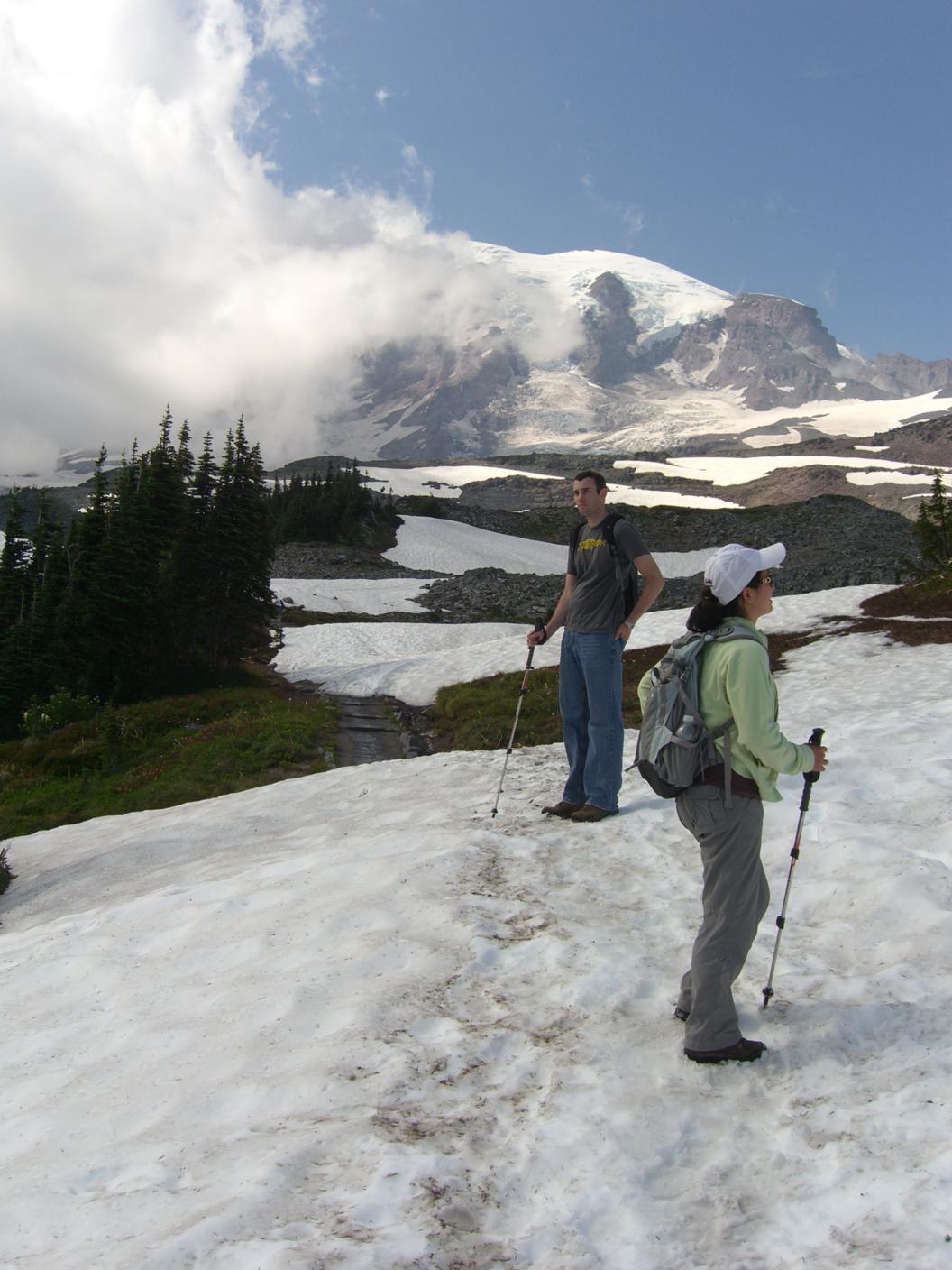
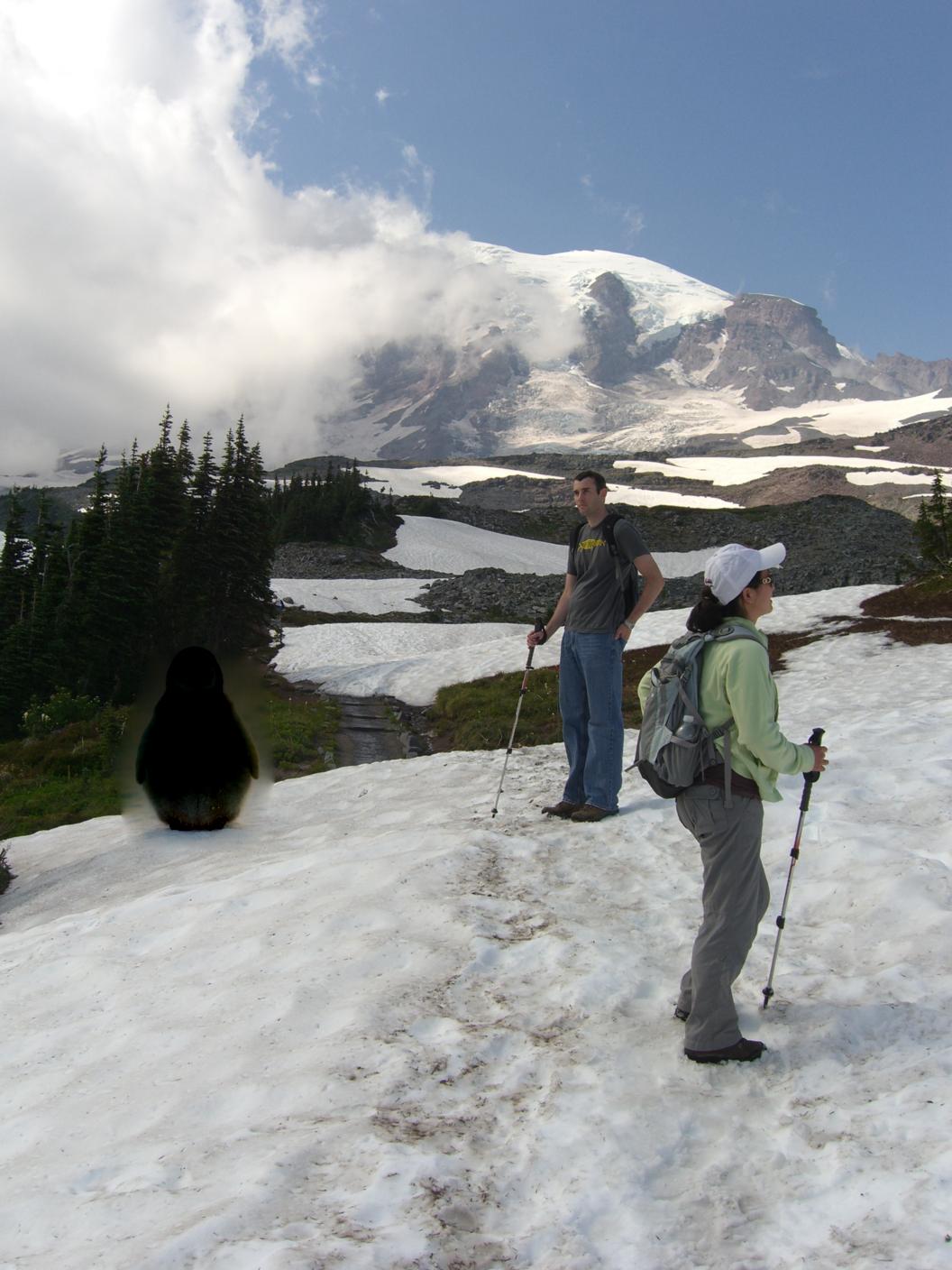
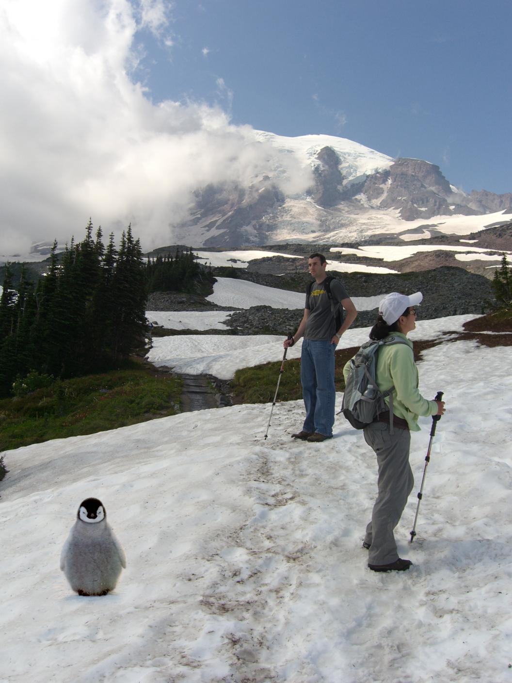
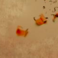
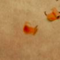
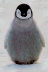
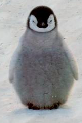
Part 2.2.3 - Poisson Blending FailureThe blending only works well if the background image is mostly the same texture and color. Here, placing the source penguin onto the tree-snow line causes a failure in the algorithm. The failure is likely due to the fact that the border contains two very distinct colors: white and green. Thus the least squares solution has a large error as it tries to resolve matching the masked region to both white and green colors. As shown, the penguin gets confused and becomes an evil penguin.
Part 2.2.4 - Comparing Frequency and Gradient Techniques
Frequency blending works best if you do not want the source image to change colors. However, textures are not preserved along the seam line. Poisson blending works best if you want to have a smooth transition of color and textures along the seam line. However, the coloring of the masked region may be unnatural. Mixed gradient blending works best if you want to preserve both the source and background textures in the masked region. However, sometimes the background textures may overpower the source textures, resulting in a unnatural image.
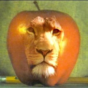
Part 2.3 - Mixed Gradients
At each pixel in the masked region, for each direction, we take the strongest gradient from either the source or background image. The result is that the masked region retains both the source's and the background's textures.
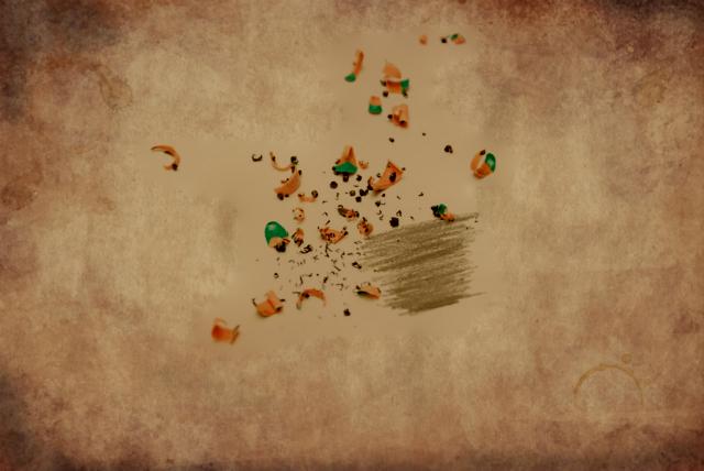
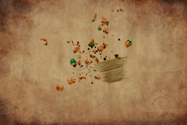
The difference is more apparent when zoomed in. For the pencil shavings picture, the Poisson blending leaves non-textured regions that are all one tone. But for the Mixed Gradient blending, the parchment paper's texture shows throughout the image, which looks much better.
Part 2.4 - Non-photorealistic Rendering - Simulated Cartoon OutlineWhenever there is an edge, there is a large gradient in an image. We detecting the pixels with large gradients and replacing them with another set pixel color, we can create outlines of images. Here, I experimented with using outlines of zero intensity pixels per channel, and with the mean of the source image per channel. That is, in the first case, when a gradient is above an empirical threshold, the pixel in that color channel is set to 0. In the second case, it is set to the average of that channel.
|