Rasterization & Anti-Aliasing

Part 1: Rasterizing Lines

My line rasterizing algorithm was based on Po-Han Lin's Extremely Fast Line Algorithm . The Algorithm is able to quickly rasterize lines with slopes in all octants of the Cartesian plane. First, the algorithm reduces the eight slope cases into four cases by ensuring the absolute value of the slope is less than or equal to 1 (by swapping x and y if dy > dx). Then it determines the directions (+/-x and +/-y) in which the line should be rasterize and the rasterization's ending iteration. The function then rasterizes the line with two separate cases: If the slope was less than or equal to 1 originally, then increment by one x-unit per iteration. If the slope was above 1 originally and then the x and y coordinates were swapped, then increment by one y-unit per iteration instead. This ensures that all pixels in a line are rasterized and no pixel is skipped because either the x-unit or y-unit was incrementing pixels faster than the other.

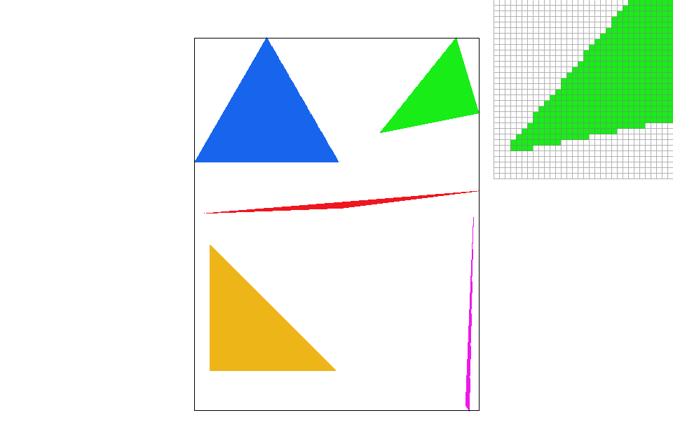
Part 2: Rasterizing single-color triangles

For both of my line-by-line triangle rasterizations, I used the rasterize_line(...) function I implemented in part 1. In my line-by-line rasterization, I first sort the vertices of the triangle (using a custom sort_vertices(...) function) and then use the sorted information to divide my triangle into two separate triangles: one with a flat top and the other with a flat bottom. For drawing each of those simplified triangles, I iterated per y-pixel and drew horizontal lines from one triangle edge to the other. My naive implementation did not have many calculations factored out and did not consider any degenerate cases. My optimized implementation did have calculations factored out and did handle degenerate cases for triangles. For example, if a triangle turned out to be a vertical or horizontal line, the optimized implementation simply called the respective rasterize_line instead.

Additionally, the naive line-by-line rasterization left many pixels not filled in. (See "Naive line-by-line.") The optimized line-by-line iterated on a sub-y-pixel level and reduced the number of unfilled pixels significantly. (See "Optimized line-by-line.")

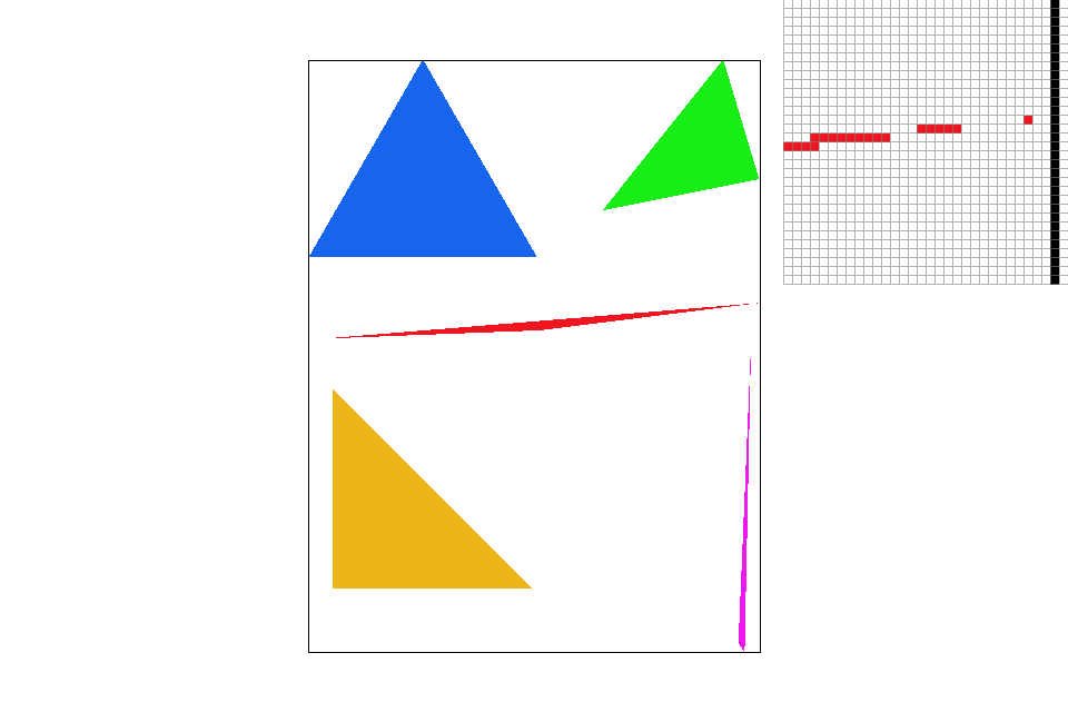
The sampling method of rasterizing triangles was also implemented. It is optimized, with many redundant calculations factored out. Also, in checking whether a sample is with a triangle, the function uses three (or less) cross products to check whether a sample is on the correct side of an edge. For checking, it calls the cross_sameside(...) function. The method of rasterizing triangles leaves no unfilled pixels along the edges of the triangles. (See "Single sampling triangles.")

Here are some timings from each of the sampling methods being used on test3.svg. To do these timings, I implemented a clock which outputs to the info string stream the time it takes to run redraw().

Naive line-by-line	Optimized line-by-line	Sampling
39.231 ms	38.283 ms	47.139 ms
41.894 ms	34.755 ms	47.945 ms
37.767 ms	36.570 ms	46.802 ms

Naive line-by-line rasterization:

Optimized line-by-line rasterization:

Sampling-based rasterization:

Line-by-line rasterization of example triangles:

Sampling-based rasterization of example triangles:

Part 3: Antialiasing triangles

I created a new buffer that is sample_rate $\times$ the size of framebuffer, called the superbuffer. At first, I tried implementing supersampling by going subpixel sample line-by-line - which turned out to be a bad idea because it made calculating the indices of each sample in superbuffer incredibly difficult and buggy. Then I decided to store samples in superbuffer on a per-pixel basis. For example, if the supersampling rate is at 16, all 16 of that pixel's samples would be taken consecutively and stored consecutively with superbuffer. This resolved all of my bugs arising from indexing errors and stopped the seg-faults. In resolve(), for each pixel, I added all sample_rate samples RGBA values together respectively and then took an naive average; and then put that rounded value into the corresponding pixel in framebuffer. (Sum of sample_rate values in a color channel divided by sample_rate.) Also, I changed rasterize_point and rasterize_line to write to the superbuffer instead of to the framebuffer directly.

A buggy implementation of super sampling and the superbuffer has a moire effect:

Supersampling, 1 sample per pixel:

Supersampling, 4 samples per pixel:

Supersampling, 9 samples per pixel:

Supersampling, 16 samples per pixel:

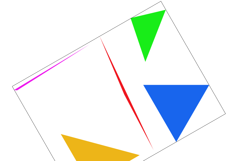
Part 4: Transforms

Implementing this part went fairly smoothly and bug-free for me. First, I implemented the three native transforms: translate, scale, and rotate. Then, I modified move_view to handle zooming and translation.

Afterwards, I added the mirrory(...) transform to transforms.cpp, which mirrors an image across the y-axis. Additionally, I added rotate_view(...) and mirror_view_y() to DrawRend. rotate_view(...) rotates the image deg degrees in place relative to the viewing screen. So, it translates the image to the origin, rotates it, and then translates it back to the center of view. mirror_view_y() flips the image across the y-axis in place relative to the viewing screen as well. So, it translates the iamge to the origin, flips it, and then translates it back to the center of view.

The images can be rotated in 30 degree increments in either clock direction using '[' and ']'. The images can be mirrored by pressing 'M'.

Triangles mirrored, rotated 60 degrees clockwise, zoomed in, translated, and supersampled at 16 samples.

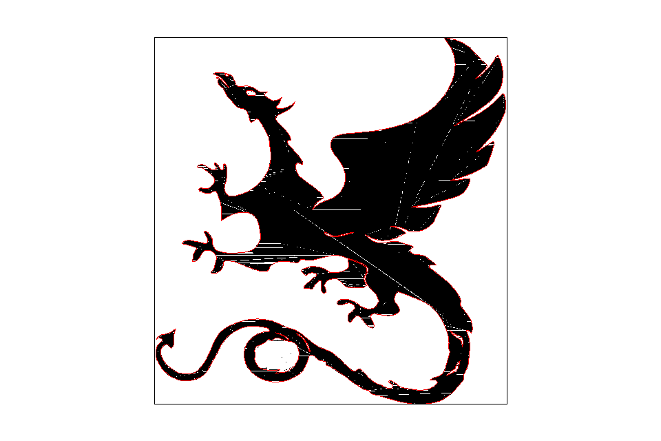
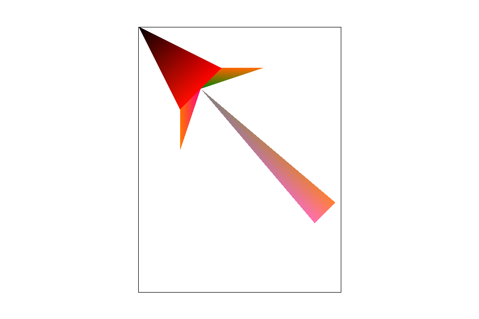
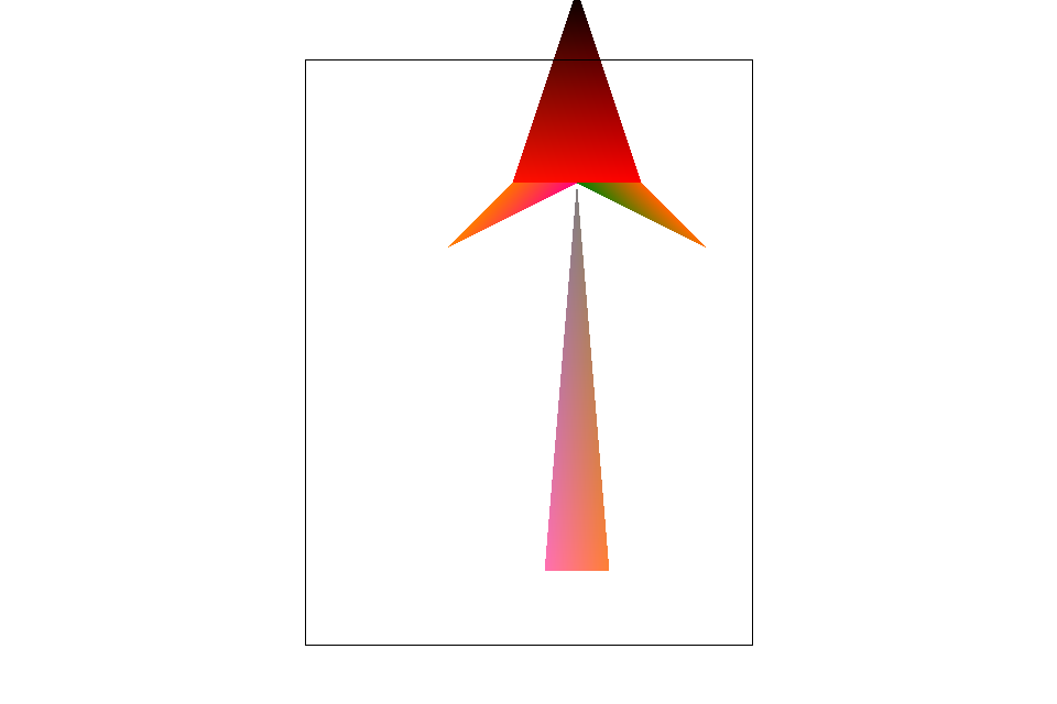
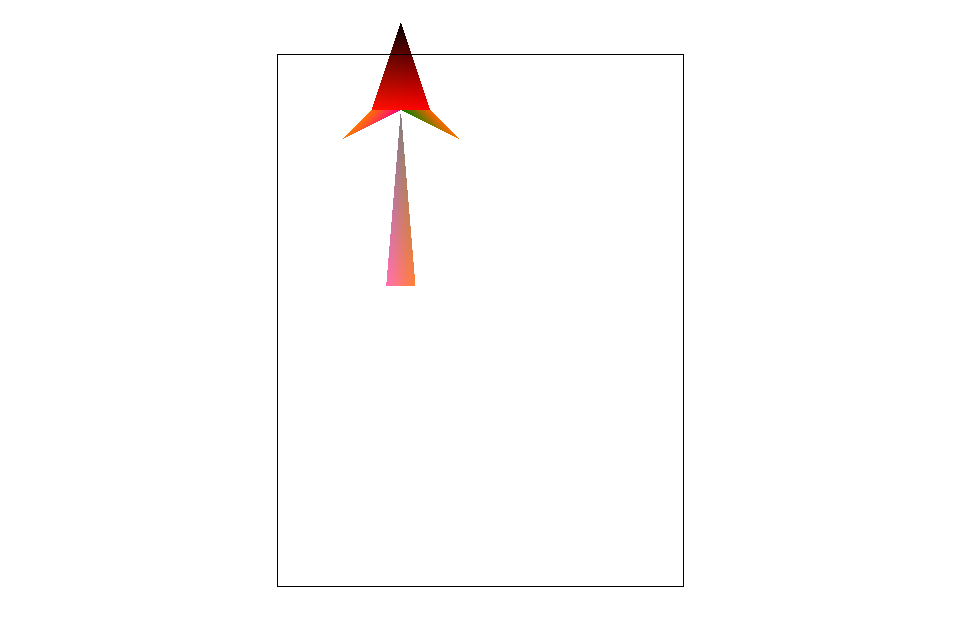
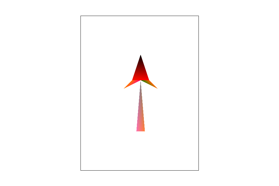
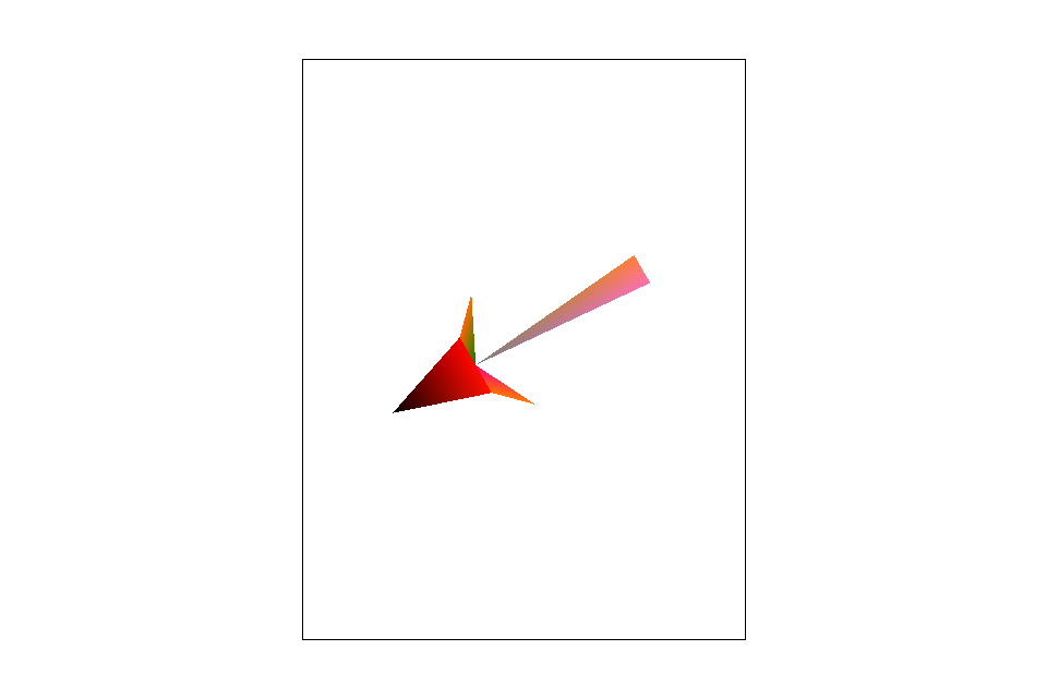
I created a new svg of a colored arrow head. It has a group of colortri's which are transformed upon.

The original image grouping $G$.

$G' = rotate(45,250,320) \times G$

$G'' = scale(0.5,0.5) \times G'$

$G^{(3)} = translate(100,200) \times G''$

$G^{(4)} = rotate(-120,240,320) \times G^{(3)}$

Part 5: Barycentric coordinates

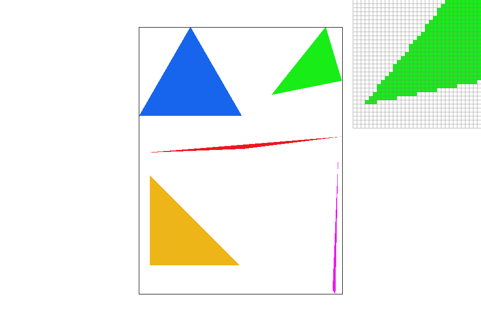
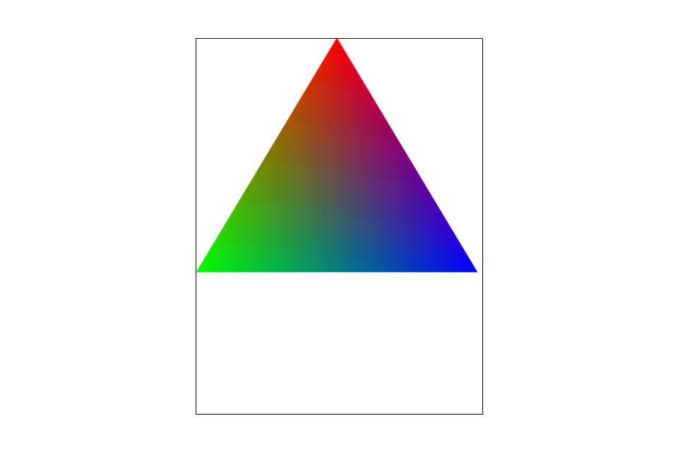
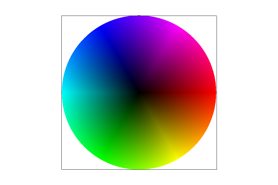
Barycentric coordinates for triangles can be thought of as an internal coordinate system for each triangle. Alpha, beta, and gamma, the coordinates of such a system, can be interpreted as weights, areas, or proportional lengths corresponding to each vertex of the triangle. The alpha, beta, and gamma values can be used for interpolating colors, textures, and possibly other characteristics within a triangle. For example, below is a triangle which has for each vertex a solid R, G, or B value. With only the color values at the vertices, the rest of the triangle can be filled with a gradient by interpolating the R, G, and B values using the barycentric coordinate system.

The transforms example above uses triangles with colors that are interpolated using barycentric coordinates too.

In implementing this function, in DrawRend::rasterize_triangle(...) I passed in the barycentric coordinates of the current sample point to tri->color if it was not NULL. Otherwise, the default color was used. In ColorTri::color(...), I extracted the alpha, beta, and gamma values from the barycentric coordinates that were passed in. Then I interpolated for the sample location's color within the triangle, and passed that color back to DrawRend for assignment into the superbuffer.

Color Wheel - This was a bug that happened when I did not reverse the normalization of the uv-coordinates correctly during the interpolation process.

Color Wheel - This was another bug that happened when I did not reverse the normalization of the uv-coordinates correctly during the interpolation process.

Example triangle with solid colors at the vertices and interpolated gradient in the center.

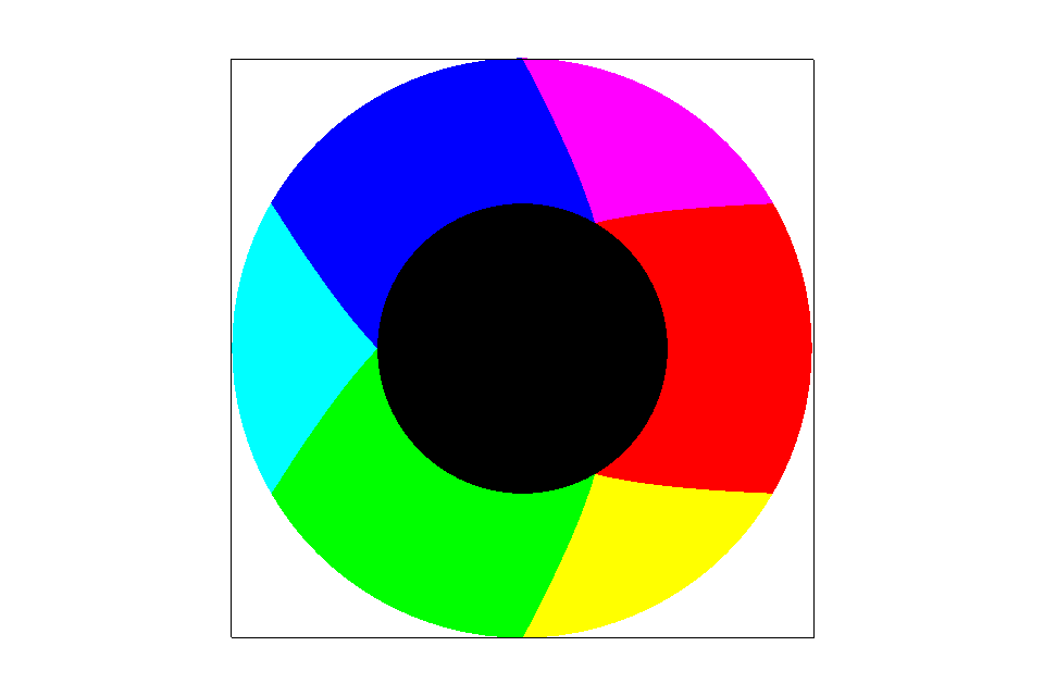
Color Wheel - With default viewing parameters and sample rate 1, now correctly drawn.

Part 6: Pixel sampling for texture mapping

First, I updated DrawRend and svg.cpp to handle switching between pixel sampling modes for texture mapping. In svg.cpp, I converted the passed in uv coordinates of xy into uv coordinates for SampleParams by interpolating the given per-vertex uv coordinates of the triangle with the barycentric coordinates. Then SampleParams was passed into tex to retrieve the texture's Color at the sampling point.

Then, I implemented Texture::sample_nearest(...) and Texture::sample_bilinear(...) for mipmap level 0. sample_nearest(...) simply returns the nearest texel to the sampling (u,v). On the other hand,sample_bilinear(...) returns the linearly interpolated colors of the four texels surrounding the sampling (u,v). Bilinear does this by first adding a weighted sum of colors for each pair of surrounding horizontal texels together. Then it (vertically) adds a weighted sum of the two previous sums together, and then returns that color.

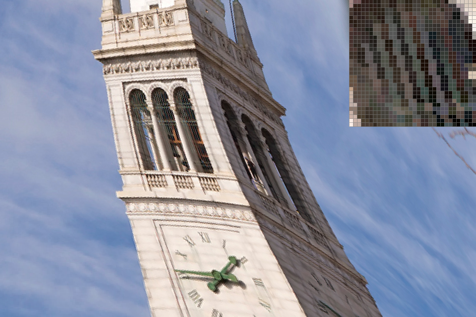
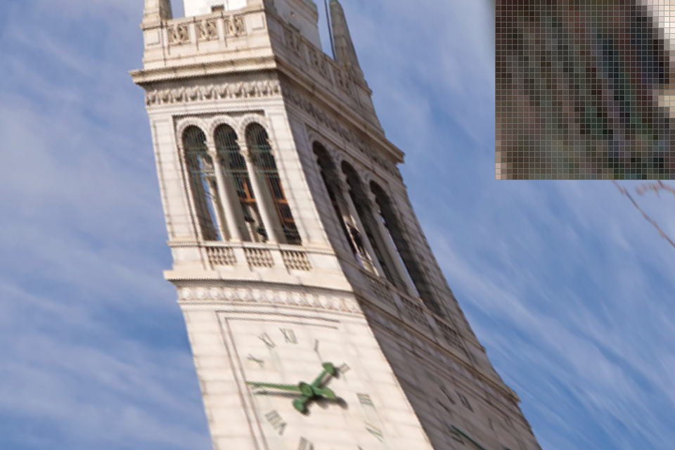
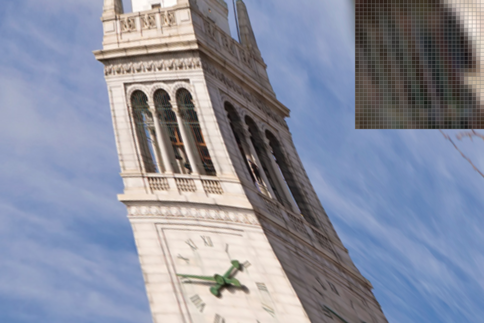
In general, bilinear pixel interpolation sampling does a much better job that nearest pixel sampling in that bilinear provides a smoother and anti-aliased image. At close to 1 pixel per 1 texel resolutions, and multiple pixels per texel (magnification), bilinear provides much better results than nearest pixel - having better anti-aliasing, less jaggies. If the image was magnified to an extreme degree however, bilinear may make the image overly blurry. Additionally when the image is zoomed out very far, meaning 1 pixel per many texels, there is little difference between nearest pixel and bilinear methods as they both do not anti-alias much.

Nearest pixel at 1 sample per pixel. Note the jaggies on the campanile's bars and on the clock hands. There is a moire effect around the ledges.

Bilinear at 1 sample per pixel. The jaggies are mostly gone, but the image in general seems a little blurry. The moire effect is reduced.

Nearest pixel at 16 samples per pixel. The jaggies are mostly gone from the capanile's bars, but the ledges and the clock's shadow still have obvious jaggies.

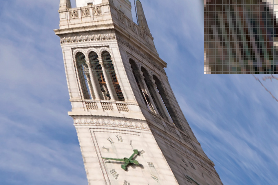
Bilinear at 16 sample per pixel. The jaggies are again mostly gone, and the image seems slightly sharper than with only 1 sample per pixel (without introducing jaggies). There is still a very slight moire effect at the top ledge of the campanile.

Neareset Pixel - There is not much difference between nearest pixel and bilinear at this zoom level.

Bilinear - There is not much difference between nearest pixel and bilinear at this zoom level.

Part 7: Level sampling with mipmaps for texture mapping

In implementing level sampling with mipmaps, I modified DrawRend to also pass in the barycentric coordinates of adjacent x-and y-sampling coordinates of the sampling point into tri->color(...). To optimize the DrawRend::rasterize_triangle(...), I only calculate and pass in those adjacent coordinates if level sampling is on. In svg.cpp, I modified TexTri::color(...) to calculate du and dv for SampleParams. To do that, first I interpolate the given per-vertex uv coordinates of the triangle with the barycentric coordinates of the newly passed in adjacent sampling locations. Then, I respectively subtract those interpolated values with the interpolated values of the base sampling location, in order to obtain the $\partial u/\partial x, \partial v/\partial x, \partial u/\partial y$, and $\partial v/\partial y$ required for computing mipmapping levels.

Then in texture.cpp, I implement the Texture::get_level(...) according to the formula provided in class. When trilinear filtering was selected (L_LINEAR), Texture::sample(...) calculates the texel value at two separate mipmap level and then interpolates between them using a weighted sum to obtain and return the filtered sample color. I optimized the level sampling methods to calculate the values for that lsm-option only when necessary. For example, only when sp.lsm == L_LINEAR do I call the sampling methods again on a higher level. Redundant calculations were factored out as well, including the square root used in obtaining the level values.

Nearest pixel and 0 level at 1 sample per pixel, at a zoomed out viewpoint.

Bilinear and 0 level at 1 sample per pixel, at a zoomed out viewpoint. The image is a little more anti-aliased as compared to the previous one.

Nearest pixel and nearest level at 1 sample per pixel, at a zoomed out viewpoint. Some choppy, moire-like effects appear around some of the edges (high frequency areas).

Bilinear and nearest level at 1 sample per pixel, at a zoomed out viewpoint. The image is relatively smooth and looks anti-aliased.

Nearest pixel and linear interpolation of two levels at 1 sample per pixel, at a zoomed out viewpoint. There is some definite artifacting occuring, and a moire effect is visible.

Bilinear and linear interpolation of two levels (Trilinear filtering) at 1 sample per pixel, at a zoomed out viewpoint. The image looks pretty smooth and well anti-aliased.

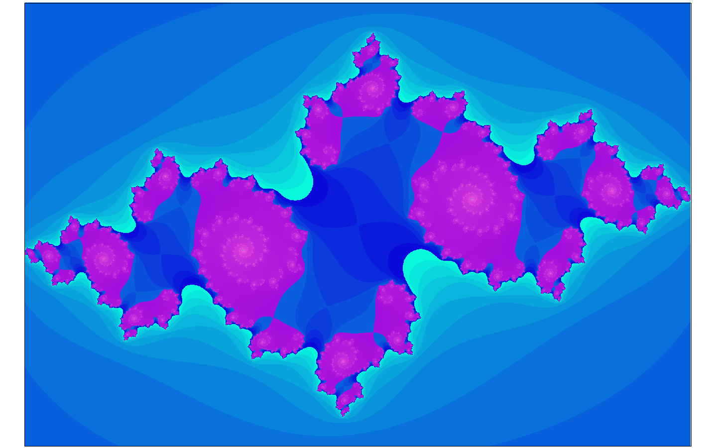
Part 8: Julia Set Fractals

With guidance from "Lode's Computer Graphics Tutorial," I implemented fractal.cpp. Executing the compiled code of fractal.cpp outputs the file fractal.svg, which is an svg file containing coordinates to a Julia set fractal. The .cpp file automatically sets up the svg/xml header and tail elements. Then, using select predefined values, it computes the Julia set's fractal, colors the appropriate pixels, and then writes that pixel's information to the svg. The svg file can subsequently be rendered using the code from earlier in the project.

Originally, I had intended for the .cpp file to take user inputs to create various color-filled polygons. That functionality can be easily implemented by replacing the print_fractal() function with another function that would take in user input. The svg head and tail elements are already taken care of by print_header() and print_header_tail(), respectively. But, I decided that was still too much work on the user end to make a draw picture. (An incredible amount of clicking and coloring.) So, I made fractals instead.

An illustration of a Julia set, generated from my fractal.cpp.